Geology Reference
In-Depth Information
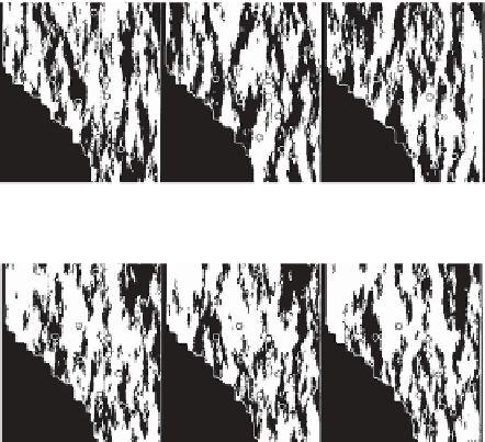
Figure 10.5
Three stochastic realisations with low impedance 'geobodies' connected to wells (after Francis and Hicks,
2010
).
approach assumes that there is no spatial dependence
of the relationship. In order to make the final map fit
the wells a residual correction surface would need to
be applied. More sophisticated approaches will be
discussed below but there are a number of issues that
the interpreter should be aware of prior to deriving a
functional dependence of seismic attributes and res-
ervoir properties. These include the role of synthetic
models, the nature of calibration and the nature of
uncertainty.
Simply crossplotting attribute values at well loca-
tions and data from the wells may not be an optimum
approach. At least in the first instance it is useful to
demonstrate the relationship between the seismic
attribute and the well data through synthetic model-
ling. At this stage careful consideration needs to be
given to the effect of facies as well as spatial controls
on any possible attribute/reservoir property relation-
ship. For example, Stanulonis and Tran (
1992
)
describe how porosity can be linearly related to seis-
mic amplitude in the Lisburne pool on the North
slope of Alaska, but find that the relationship varies
in separate geographical regions due to factors such as
sub-cropping geology, the presence of fractures and
variation in fluid phase (i.e. oil vs gas). Another issue
to investigate in determining a seismic/rock property
function is the uncertainty that arises from the limited
resolution of seismic. For example, beds below a
certain thickness might not be evident on seismic
but these beds may be effective reservoir and may
have been used to calculate rock property values from
well logs.
Following the determination of an attribute/rock
property relationship using synthetics the next step is
calibration of well and seismic values. When cross-
plotting mapped seismic attribute and well property
data there is inevitably a question over which value to
take from a seismic map: is it the closest value, an
a)
channel
non-channel
1km
b)
Figure 10.6
Channel sand models generated for the Ness
formation in Oseberg Field, Offshore Norway using wells and seismic
amplitudes. N-S and E-W correlation ranges are (a) 1000 m and
600 m and (b) 2000 m and 600 m respectively. After Doyen et al.,
1994
. Copyright 1994, SPE. Reproduced with permission of SPE.
Further reproduction prohibited without permission.
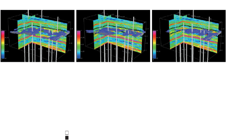
discrimination of fluids (
Fig. 10.7
). P-impedance,
S-impedance and density were inverted from pre-
stack gather data using a model based inversion
approach (
Figs. 10.8a
-
c
). Empirical transforms based
on the available well data were used to predict rock
properties from the inverted products. N:G, porosity
and water saturation maps are shown in
Figs. 10.8d
-
f
.
10.3.2 Simple regression, calibration
and uncertainty
In many cases the simplest approach in mapping
reservoir properties from seismic is to apply a trans-
form to the seismic attribute map based on cross-
plotting of seismic and well data (
Fig. 10.9
). This
226