Geology Reference
In-Depth Information
a)
b)
6000
Density
(g/cc)
West
East
AI
AI
Abu Sir 2X
6000
8000
8000
2.4
GR Res
2.3
2.2
2.1
2.0
GWC
GWC
Low saturation gas
Figure 9.27
Density inversion at a well, showing commercial
gas saturations in red and yellow colours and low gas saturation/
non-gas responses in green (after Roberts et al.,
2005
).
Other stochastic methods, such as the Bayesian inver-
sion technique of Gunning and Glinsky (
2003
), are
more closely constrained to layer thicknesses deter-
mined by the bandwidth of the data.
Figure 9.30
illustrates an example of several imped-
ance realisations, all fitting at the wells and honouring a
geostatistical model determined from well data and a
lateral spatial variability model. Note that following the
discussion of angle-dependent impedance and angle-
independent elastic parameters presented in
Chapter
5
, the term
20m
is used here in a generic sense
to represent any quantity inverted from seismic (i.e.
including V
p
/V
s
ratio).
Figure 9.31
shows a typical
example of a single stochastic impedance realisation
and also the mean and standard deviation of a large
number of realisations. The smoothness of the mean
solution (
Fig. 9.31b
) compared to the single realisation
(
Fig. 9.31a
) is a general feature of all stochastic inver-
sions as is the increase in the standard deviation (
Fig.
9.31c
) away from the well control, consistent with
honouring the data at the well.
An analysis of stochastic realisations can typically
provide:
(1) probability of a particular facies occurring at a
given location, for example oil sands having an
impedance below a particular threshold,
(2) statistical distributions of volumes and areas,
(3) indications of likely connectivity, for example,
whether a particular area of low-impedance gas
sand samples is likely to be connected to a well
penetration.
'
impedance
'
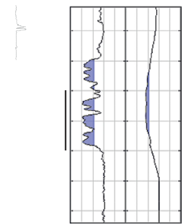
Figure 9.28
The effect of log upscaling on estimating sand
thickness in thin beds; (a) 0.152 m (raw log) sampling (b) 20 m
Backus average. Blue zones are values below an impedance value of
6865 m/s.g/cc, characterising sand. Note how applying the
threshold to the upscaled log (simulating the seismic scale) gives an
underestimate of sand thickness. Horizontal depth lines are 10 m.
to simultaneous realisations of facies and reservoir
properties conditioned by a geo-seismic model and
presented within a depth referenced geo-cellular grid.
Stochastic inversion is a rapidly developing area of
geophysics and the discussion presented below
attempts to outline the key elements and approaches.
The reader is referred to the work of Dubrule (
2003
)
and Bosch et al.,(
2010
) for useful reviews.
The first successful application of geostatistics in
seismic inversion was presented by Haas and Dubrule
Numerous workflows exist in stochastic inversion,
from inversions that utilise geostatistics to generate
multiple realisations of impedance in the time domain
215