Geology Reference
In-Depth Information
a)
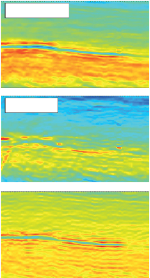
Figure 9.26
Typical results from
simultaneous inversion; (a) acoustic
impedance, (b) shear impedance and (c)
density. Note that the low AI and density
layer is a hydrocarbon sand (courtesy Ikon
Science).
10000
1700
Acoustic Impedance
9000
1800
8000
7000
1900
6000
5000
2000
b)
6000
5500
5000
4500
4000
1700
Shear Impedance
1800
1900
3500
3000
2000
2500
c)
3.0
Density
1700
2.75
2.5
1800
2.25
1900
2.0
1.75
2000
1.5
the effect of lowering the gross rock volume in the
closure as well as enhancing the connectivity.
seismic as well as honouring both the well data,
the statistical properties of the impedances as well
as any spatial model constraints. Given a sufficient
number of realisations, the mean is close to the deter-
ministic or best estimate inversion.
Stochastic inversions that utilise geostatistics (i.e.
geostatistical inversions) typically use a small sam-
pling increment (e.g. 1 ms) allowing the inversion
results to be integrated with reservoir models. Indeed,
experience has shown that integrating the seismic into
geological models using geostatistical inversion tech-
niques enables greater control on the uncertainties in
reservoir models (e.g. Rowbotham et al.,
2003b
).
9.3 Stochastic inversion
Whilst deterministic or best-estimate inversion
obtains a minimised solution of the inverse problem,
stochastic inversion techniques attempt to describe
the potential variability of inverse solutions. Unlike
deterministic inversion, therefore, a stochastic inver-
sion does not provide a single
solution.
Multiple realisations of the subsurface impedance
are generated, the synthetics from which all tie the
'
optimal
'
214