Geology Reference
In-Depth Information
1210
1250
1300
1350
1400
1450
1500
1.5
1.8
1 km
Figure 9.5
Example of model-based inversion; horizon picks on reflectivity data, used to establish initial model (after Pharez et al.,
1998
).
200ms
200ms
5000
5833
6667
7500
Impedance
4372
5565
6764
7960
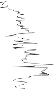
Figure 9.6
Example of model-based inversion; well impedance
(black) and macro-layering starting model for the inversion (red).
Impedance
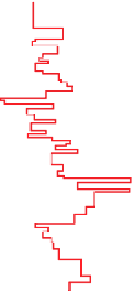
Figure 9.7
Example of model based inversion; micro-layering
output from the inversion (red), well impedance (black).
There are two important approaches to the
checking of an inversion. These are impedance pre-
diction at wells and synthetic
seismic error plots. If
the initial model was created using the well as input,
then the match is always likely to be good. A better
test is to use a
-
validation
. Blind well tests are only sensible, however,
if there are a fairly large number of wells in the project
area. If there are only two or three then the omission
of one of them greatly loosens the constraint on the
model.
Figure 9.9
shows an example of a blind well test.
'
well, not incorporated in the
initial model. This is sometimes referred to as
'
blind
'
202
'
cross