Geology Reference
In-Depth Information
observed velocities (e.g. Wild,
2011
). Whilst anisot-
ropy is often of secondary importance in calculating
reflectivities for well ties, the interpreter should con-
sider the possibility that incorporating the anisotropy
into the reflectivity calculation may improve the tie,
particularly if the seismic has been processed using an
anisotropic velocity model. In the case of HTI scen-
arios, reflectivities need to be calculated for the cor-
rect azimuth.
4000
4000
3500
3500
3000
3000
2500
2500
2000
2000
1500
1500
1000
1000
500
500
0
10
10
20
20
30
30
40
40
50
50
60
60
70
70
80
80
90
90
0
8.5 Practical issues in fluid substitution
The application of Gassmann
Well deviation angle (degrees)
Well deviation angle (degrees)
'
s equation is compli-
cated by the fact that real rocks deviate from the
simple assumptions inherent in the model. Three
commonplace fluid substitution scenarios which
require careful thought are shaley sands, laminated
sands and tight (gas) sands. There are pitfalls for the
unwary. The reader is referred to
Sections 8.2.3
and
8.2.5
for background discussions on Gassmann
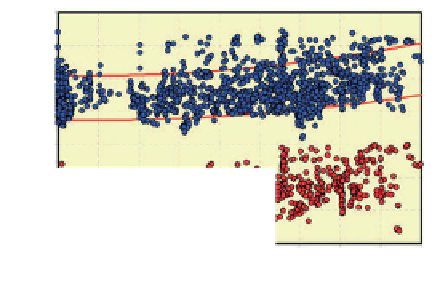
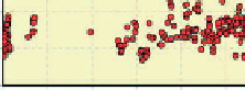
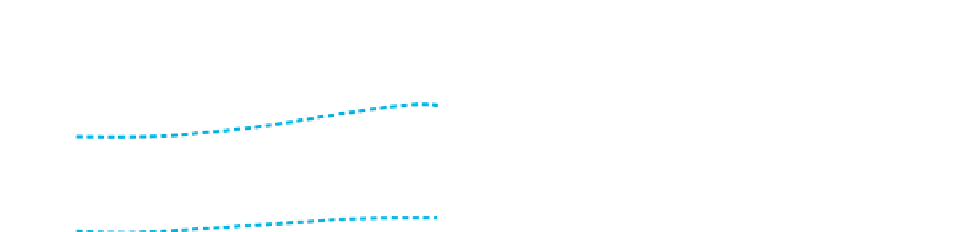
Figure 8.57
Well log velocity data from pure shales in 10 shale
formations in two North Sea fields (after Brevik et al.,
2007
). Red lines
indicate +/ 12.5% P wave velocity variations relative to a trend of
velocity with deviation angle. Dashed blue lines are velocity
predictions based on Thomsen's(
1986
,
2002
) anisotropic equations
(
Chapter 5
) using δ ¼ 0.05, ε ¼ 0.18 and γ ¼ 0.18.
'
s
properties and environmental conditions. The impli-
cation is that a variety of fits may be possible but at
least it gives a basis for making a correction that can
be tested by a well tie. The volume of shale log is used
to apply the correction (assuming that clean sands
are essentially isotropic, e.g. Wang,
2001a
,
b
). Differ-
ent authors have used slightly different functions and
shale cut-off points but in general no correction is
necessary up to 20%
equation and dry rock trends.
8.5.1 Shaley sands
A common pitfall in the fluid substitution of shaley
sandsisanexaggeratedsubstitutioneffectonthe
compressional velocity and Poisson
s ratio logs in
low-porosity shale prone zones (e.g. Skelt,
2004
;
Simm,
2007
).
Figure 8.58
shows a typical example
where gas has been substituted for water. Note how
the Poisson
'
30% V
sh
, whereas the full
correction should be applied beyond 70%
-
80% V
sh
.
In between these cut-offs the correction can be
applied linearly.
Any data that might be used to derive anisotropic
parameters, such as walk away VSP results, aniso-
tropic velocity measurements on core samples and
anisotropic information from time and depth pro-
cessing, might be useful in constraining the aniso-
tropic model. When there is only a single deviated
well with a standard suite of logs, the issue becomes
one of trial and error (i.e make a correction based on a
generalised idea of the anisotropy and evaluate the
resulting well tie). Empirical approaches, such as those
presented by Ryan-Grigor (
1997
) (see
Chapter 5
) and
by Tsuneyama andMavko (
2005
), might be used as the
basis for an initial estimation of
-
s ratio log in places is close to zero and
how some of the shaley zones have a greater mag-
nitude of P wave fluid substitution effect compared
to the clean sands. Intuitively this is incorrect. In
this particular case the porosity input
'
to Gass-
mann
s equation is effective porosity (derived from
the density log using a mix of shale and quartz) and
the effective mineral modulus is derived by mixing
shale and quartz using the Voigt
'
-
-
Hill aver-
age (see
Section 8.2.1
), with shale parameters being
estimated from the logs. The normalised modulus
plot (see
Section 8.2.3
) shows that the clean sands
have reasonable dry rock values (
Fig. 8.59
), but
as the shale volume increases so does the scatter
on the plot. Below about 8% porosity, some of the
bulk modulus points are negative, which is not
physically possible. Many of the high V
sh
points
are plotting as very soft material, which leads to
the large fluid substitution effects on the compres-
sional velocity log.
Reuss
the anisotropic
parameters.
The analysis of log data from deviated wells in
which horizontal transverse isotropy (HTI) is present
(i.e. vertical fractures) follows a similar workflow in
which HTI anisotropic theory (e.g. Hudson,
1981
;
Schoenberg and Sayers,
1995
) is used to justify
192