Geology Reference
In-Depth Information
a)
b)
6000
Castagnas
sandline
7000
Castagnas
sandline
5500
6500
5000
6000
4500
Castagnas
mudline
5500
4000
5000
3500
4500
4000
3000
7000
8000
9000
10000
11000
9000
10000
11000
12000
V
p
(ft/s)
V
p
(ft/s)
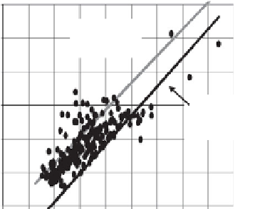
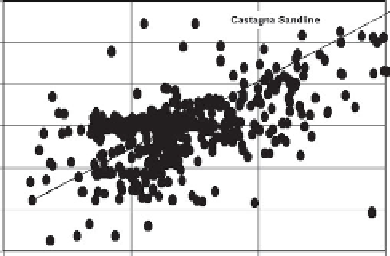
Figure 8.47
Crossplots of velocities from sonic waveforms; (a) an early example of dipole sonic data in shales with shear velocities lower
than the compressional velocity of mud. Note the presence of some mud arrival energy at around 4500 ft/s, (b) an example of dipole sonic
data example from sandstones showing mud arrival energy and significant noise.
a)
b)
Original processing
Re-processing
2500
2500
2000
2000
1500
1500
1000
1000
Sand
Sand
Shale
Shale
500
500
1000
2000
3000
4000
5000
1000
2000
3000
4000
5000
V
p
(m/s)
V
p
(m/s)
Figure 8.48
An example of Stoneley wave interference, biasing interpreted shear wave velocities to lower values. This effect can only
be established with detailed phase analysis.
are largely unusable but fortunately the fidelity of
modern sonic tools is such that this situation does
not often arise.
There are some sonic effects that cannot be recog-
nised simply by looking at crossplots. For example,
interference from Stoneley waves can bias the V
s
log
towards lower velocities.
Figure 8.48
shows an
example. It is also possible for a positive bias to be
introduced owing to interference of the shear wave
with compressional arrivals. Such effects can only be
picked up by detailed phase analysis of the waveform
data (e.g. Kozak et al.,
2006
).
185