Geology Reference
In-Depth Information
GR
DT
ρ
V
cl
DTCO
CAL
Phi
e
CAL
V
Phi
ρ
70
170 0
1 0.3
0 1.95
2.95
140
40
8
12
50m
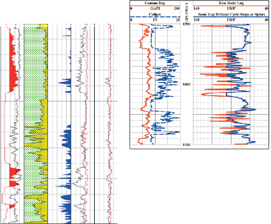
Figure 8.45
The effect of cycle skips on conventional sonic logs
(after Burch,
2002
; AAPG ©2002, reprinted by permission of the
AAPG whose permission is required for further use). The raw sonic
log (red curve, right track) shows cycle skips and noise correlating
with an enlarged borehole (note caliper log, blue curve left track).
5500
5000
Log data
4500
Figure 8.44
Example of shale 'washout'zones on density and sonic
logs. Predicted density log is shown in red in column 4. Note how
the dipole compressional sonic log (DTCO) is less affected by the
washouts than the conventional sonic (DT).
4000
3500
Shale Line
3000
7500
8000
8500
9000
An initial QC of compressional and shear logs
should include checking the Poisson
P Wave Velocity (ft/s)
sratioorV
p
/V
s
log for anomalously low or high values. Other errors
can be picked up on V
p
vs V
s
crossplots but not all. If the
semblance data are available it is worth reviewing these
to check the picks. Monopole tools have the limitation
that where the shear velocity of the formation is less
than the compressional velocity of the drilling mud
(
'
Figure 8.46
Example of monopole array sonic data showing mud
arrivals masquerading as shear arrivals in a
'
slow
'
formation.
sonic.
Figure 8.47a
shows an example of dipole data
in shales from the mid 1990s, with the shale data
mostly located where
they might be
expected,
formations), no shear wave is recorded and
instead the tool will tend to record the mud velocity.
This is easily detected on a V
p
vs V
s
crossplot, where
the shear velocity will be roughly constant and higher
than that expected from empirical trends such as
Castagna
'
slow
'
between Castagna
s mudline and sandline. However,
there is still some interference from mud arrivals at
velocities around 4500 ft/s. This would require
editing or possibly more appropriately to use the
dipole data to determine linear empirical fits for V
s
prediction.
Figure 8.47b
shows an example of poor
dipole data in sands, with mud arrival energy and
significant scatter in the shear direction. These data
'
s mudline or sandline (
Fig. 8.46
).
The mud arrival problem in slow formations was
largely solved with the development of the dipole
'
184