Geology Reference
In-Depth Information
b)
a)
3
3
40%
shale
30%
2.8
2.8
30%
2.6
20%
2.6
(1)
2.4
2.4
10% porosity
20%
(3)
(4)
(6)
2.2
2.2
brine sand
brine sands
oil sands
shale 1
shale 2
shale model
oil sand model
brine sand model
10%
40%
clean sand
2
2
30%
35%
30%
20%
25%
1.8
1.8
10% porosity
Gas saturation
10%
100%
20%
(2)
15%
(5)
1.6
1.6
1.4
1.4
2000
4000 6000 8000 10000
Acoustic impedance (m/s.g/cc)
2000
4000 6000 8000 10000
Acoustic impedance (m/s.g/cc)
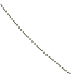
Figure 8.43
Rock physics template examples; a) a template crossplot showing the rock physics illustrating the vectors associated with certain
elastic changes relative to a reference brine sand: (1) increasing laminar shale, (2) increasing cementation, (3) increasing porosity, (4) decreasing
effective pressure, (5) increasing hydrocarbon saturation, (6) increasing dispersed shale content (modified after
degaard and Avseth,
2004
),
(b) an example of log data plotted from different lithofacies zones, together with rock physics model calibration trends.
ties. Log editing is therefore an important element of
the well tie process. Typical causes of bad hole condi-
tions are the presence of incompetent formations and
chemical interaction of mud filtrate and clays. In
many instances the caliper log is a key to recognising
bad hole. The density tool in particular has low toler-
ance of poor hole conditions.
Figure 8.44
shows an
example of zones of caving shales that have led to
errors in the density log. In this instance a corrected
log has been calculated by using sand and shale dens-
ities, mixed in the proportions indicated by the V
cl
log. Such a scheme is valid of course only where the
fluid fill is invariant and there is no depth dependency
in the density and sonic measurements.
In contrast to the density log, wireline sonic logs
are usually quite tolerant of poor borehole conditions.
However, in very bad hole the sonic signal, particu-
larly with conventional borehole sonic logs, can be
severely attenuated. This results in the amplitude of
the first arrival being too low to trigger the receiver,
which instead records higher amplitude later arrivals.
This
tolerant of bad hole than older designs (
Fig. 8.44
).
Sometimes sonic logs also show noise spikes where
the receivers are triggered by, for example, tool move-
ment. Log spikes deserve careful attention to distin-
guish noise from genuine responses for example
related to thin limestone stringers in a shale section.
Comparison with other logs such as density is usually
helpful. It is also worthwhile checking for potential
bad hole effects on the seismic drift curve generated
during log calibration (
Chapter 4
). The bad hole will
show up as zones in which sonic velocities are slower
than seismic velocities.
8.4.2 V
p
and V
s
from sonic waveform
analysis
Since the early 1990s shear wave logging has become
fairly routine. As discussed in
Section 8.3.2.2
,com-
pressional and shear logs are derived from an analysis
of sonic waveforms. In general, rig-based processing
products are not the best quality. Final logs are
generated from detailed analysis in a dedicated pro-
cessing centre. In projects where there are a number
of wells with variable age shear logs, interpreted by
different contractors, it is unlikely that the interpret-
ations will be consistent. In such a situation it is well
worth considering re-processing all the wells to obtain
a consistent dataset prior to the start of the project.
can lead to sonic transit times
that are too high (i.e. velocities too low) (
Fig. 8.45
).
In
Fig. 8.45
the effect of cycle skips in bad hole has
been corrected by defining a relationship between
deep conductivity (i.e the reciprocal of the deep resist-
ivity log) and sonic slowness (Burch
2002
). Modern
dipole and other advanced sonic tools are more
'
cycleskipping
'
183