Geology Reference
In-Depth Information
shared dependence of resistivity and sonic measure-
ments on porosity. Faust (
1953
) was effectively the
first worker to propose a usable relation:
1
6
,
¼ γ
ðÞ
ð
:
Þ
V
p
ZF
8
14
where V
p
is in ft/s with
γ ¼
1948 and Z in feet, or V
p
is
in km/s with
γ ¼
2.2888 and Z in km, and F
¼
resist-
ivity formation factor (R
t
/R
w
), R
t
¼
deep formation
resistivity and R
w
¼
resistivity of water, and resistiv-
ity units are ohm-metres.
A useful way of looking at Faust
s relation is that
it is effectively a scaling function of the resistivity
combined with a low frequency trend, in this case
determined by depth. In the absence of a significant
depth-related trend, scale functions are readily derived
and applied. A number of different resistivity
'
-
sonic
relations have been proposed:
a+bR
1
=
c
t
¼
ð
8
:
15
Þ
(where t is in
s/ft, and a,b and c are determined from
the data) is known as the
μ
'
-
'
Kim
Rudman
equation,
after Kim (
1964
) and Rudman et al.(
1975
);
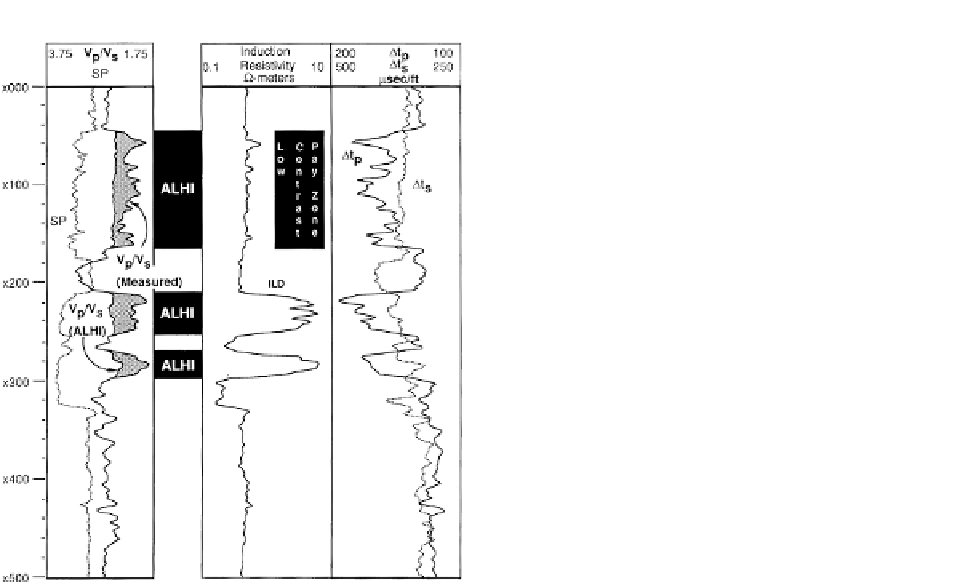
Figure 8.13
V
p
-V
s
relations to determine
pay zones (after Williams,
1990
). Column 1
An example of using
differences
between the AHLI attribute and V
p
/V
s
(measured) are shaded
grey and represent zones that the ALHI technique would predict
to be hydrocarbon-bearing. Note that the shaded areas in the
low-contrast pay zone are as definitive of the hydrocarbon-
bearing interval as they are in the cleaner zones deeper in the
well. Column 2 - resistivity logs showing low resistivity zone
around × 100. Column 3 - compressional (Δt
p
)andshear(Δt
s
)
sonic logs.
-
aR
b
,
t
¼
ð
8
:
16
Þ
where a
s/ft and resistivity in
ohm-metres. This is generally known as Smith
¼
94.2, b
¼
0.15, t is in
μ
'
s equa-
tion (Adcock,
1993
).
It is important that these types of scaling func-
tions are verified from wells with both sonic and
resistivity and that due attention is paid to stratig-
raphy, lithology and pore pressure as well as the
presence of erroneous log responses due to bad
hole or other factors (see
Section 8.4.1
). It is also
important to recognise that the functions will fail
in hydrocarbon zones. Which resistivity log to use
is essentially a data dependent decision. The resist-
ivity log needs to have a similar character to the
sonic log for scaling functions to be successful
ofcourse.IntheGulfCoastregiontheSFLlog
(shallow investigating Spherically Focussed Log)
appearstobemoreappropriateforaonestep
resistivity
(1) Calculate sandline V
p
/V
s
¼
1.182 + 0.00422 dts
(where dts
¼
shear sonic slowness in
μ
s/ft).
(2) Calculate shaleline V
p
/V
s
¼
1.276 + 0.00374 dts.
(3) Calculate water-bearing minimum V
p
/V
s
¼
min
[V
p
/V
s
(sand), V
p
/V
s
(shale))]
-
0.09.
(4) Calculate ALHI
water-bearing min V
p
/V
s
-
measured V
p
/V
s
. Whilst the AHLI attribute is not
especially sensitive to saturation (especially with
gas), it can be particularly useful in indicating the
presence of pay in low resistivity situations.
¼
sonic transform than the deep induction
ILD log (Smith,
2007
)(
Fig. 8.14
). However, in other
areas borehole effects such as mud filtrate invasion
may be an important issue to address in the choice
of resistivity log.
A more petrophysical approach, effectively based
on Wyllie
-
8.2.2.5 Faust's relation
In wells that do not have a sonic log it is common
practice to transform resistivity to sonic for the pur-
poses of seismic horizon ties, particularly in areas
where the geology is dominantly a passive fill
sequence. The basis for the transformation is the
s relation, has been described by Fischer
and Good (
1985
):
'
158