Geology Reference
In-Depth Information
soft response at the top of the gas sand. The inter-
preter should also check for a dim spot effect on the
near
a)
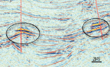
King Kong (Gas) GC473
Lisa Ane (Fizz) GC474
stack to further
justify the hydrocarbon
interpretation.
Figure 7.12
shows an example which illustrates the
value of the far stack for hydrocarbon identification
in this AVO scenario. The top of the hydrocarbon-
bearing oil sand reservoir is clear on the far stack
(
Fig. 7.12b
), being the high amplitude soft black loop.
On the nears (
Fig 7.12a
) it is difficult to see the subtle
dimming of the hard red/orange loop that would be
consistent with the presence of oil. The phase reversal
shown on the gather (
Fig. 7.11c
) emphasises the need
for accurate velocity analysis to correct for normal
moveout.
The philosophy of using simple models to aid
interpretation is illustrated very well by the example
shown in
Fig. 7.13
, which led to an oil discovery in the
Gulf of Mexico (Ross,
1995
). In this case, the rock
physics analysis done as part of the exploration effort
suggested that oil sands would have Class IIp
responses whilst wet sands would have Class
I responses. It was realised that if the near stack was
crossplotted against the far stack the oil sand reflect-
ivity (top and base) would fall in particular areas of
the plot (
Fig. 7.13a
). Colour coding the data on the
seismic sections (
Fig. 7.13b
) enabled the identification
of a major Class IIp anomaly that could be mapped
over a large area and which had good geological
justification.
AVO projections can be used to good effect in
this AVO scenario. Whitcombe et al. (
2002
) illus-
trate the mapping of fluid and lithology effects using
a modification of the Shuey equation (
Chapter 5
).
The lithology and fluid maps shown in
Fig. 7.14
were generated by using intercept and gradient
bandlimited impedance volumes that were combined
at AVO (
4
5
W
E
b)
+
Effective Angle
Shale/wet sand
Shale/gas sand (30% Sw)
-
Shale/sand (95% Sw)
Figure 7.8
Soft amplitudes related to variable saturations of gas; (a)
seismic sections (after O
Brien,
2004
) showing no significant
differences between a discovery well and a well with low gas
saturation, (b) top sand AVO plot generated from published log data.
'
The clearest feature on the full stack migrated
section is a bright peak reflection related to the
response from the gas water contact whilst the top
of the reservoir does not have a distinct reflection.
A notional AVO model consistent with these obser-
vations is shown in
Fig. 7.11b
. The presence of a
hydrocarbon accumulation is demonstrated by the
apparent thickening of the isochron between the
bright peak and the peak above. The time thickness
of the pay zone can be estimated by the extra
thickening observed. Of course in exploration rec-
ognising these effects requires careful observation of
the seismic signatures combined with a rock physics
model developed from appropriate well information.
In all likelihood the correct interpretation would be
clearer on the far stack where (as indicated by the
rock physics model in
Fig. 7.11b
) the base reflection
would be even brighter but would be matched by a
51.3°) and 12.4°
respectively. The oil water contact is shown as the
blue outline. Note how the lithology volume effect-
ively cancels the fluid effect in the data revealing
the channel shapes which crosscut the contact,
whereas the red areas on the fluid map reveal the
presence of oil sands. The misfit of the red colours
with the oil water contact in the west is due to poor
data quality in this part of the field.
Figure 7.15
shows some examples of these types of fluid and
lithology cubes, with schematic AVO crossplots
illustrating the mechanics behind their generation
(see
Section 5.5
).
χ
) angles of 308.7° (or
132