Geology Reference
In-Depth Information
may not be possible to confidently discriminate wet
sands from hydrocarbon sands.
Figure 7.4
shows an example of the use of colour
coded crossplots from an area with Class III gas and
water sands. Intercept and gradient have been plotted
for samples within a time window around the zone of
interest. Various clusters of samples have been high-
lighted in different colours and posted on the seismic
section. It is expected that the tops of hydrocarbon
sands will plot to the lower left and the base of
hydrocarbon sands or hydrocarbon contact reflec-
tions will plot in the upper right (
Chapter 5
). The
points highlighted with the yellow and blue colours
are therefore of interest. On the seismic section it
is evident that these points fit with the structural
culmination on the seismic section, supporting the
interpretation of a hydrocarbon sand.
A common pitfall in this AVO scenario is misin-
terpreting
structural closure, nor does it have the characteristics
of a geologically plausible trap (
Fig. 7.5c
). Without a
connection of the amplitudes to a trap, the interpreter
should be wary of assigning a DHI interpretation.
The anomaly shown in
Fig 7.6
is also accentuated
by tuning effects (
chapter 5
), a common pitfall in
scenarios where brine sands give soft seismic
responses. In these types of situations it may be
impossible to distinguish between a productive pay
interval and a water bearing sand.
Fig 7.6
shows an
example where a productive gas zone and a thin water
wet sand produce similar AVO responses. Such obser-
vations are useful in the risking process (
Chapter 10
)
.
AVO exploration is most successful in areas where
the background geology is laterally invariant and the
hydrocarbon signatures stand out from the back-
ground. Variations in lithology can give rise to ambi-
guities in the interpretation of AVO signatures.
Figure 7.7
illustrates an example in which there are
both variations in fluids (water and hydrocarbons)
and a dominant facies change from clean sand to
shaley sand. The coloured segments from the sche-
matic section (
Fig. 7.7a
) represent zones with differ-
ent AVO signatures (
Fig. 7.7b
). The clean sands in the
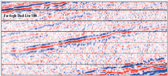
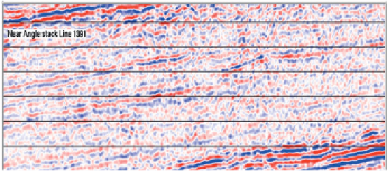
from water sands as a hydro-
carbon effect.
Figure 7.5
shows an example. The AVO
effect is dramatic on the partial stacks (
Fig. 7.5a
) and
the seismic gathers (
Fig. 7.5b
) but it is caused by a
thin shaley water bearing sand. In this instance, the
amplitude effect shows no obvious consistency with
'
rising AVO
'
a)
b)
offset
Near angle stack
100ms
100ms
A
I
c)
=
Low
Far angle stack
High
100ms
High
129
Figure 7.5
A Class III AVO response caused by a water bearing shaley sand; (a) near and far angle stacks, (b) gather example, (c) map showing
monocline structure and zone of high amplitude with no obvious consistency with structure. Tuning is contributing to the high amplitude.