Geology Reference
In-Depth Information
a)
b)
Intercept
3
1
2
3000
5
0
-5
Gas
3200
3400
2500
4
5
6
Oil
2600
2700
2800
2900
Gradient
3000
7
8
9
2
0
-2
Brine
3200
3400
2500
10
11
12
Shaly sands
and brine
2600
2700
2800
2900
Gradient/intercept
1
Top reflector
(shale = cap)
Base reflector
(shale = base)
Base reflector
(shaly sand = base)
(3, 6, 9)
Shale-shale
interface (12)
0.5
0
0.5
-1
-0.5
-0.4 -0.3 -0.2 -0.1
0
0.1
0.2
0.3
0.4
0.5
c)
no class
shale
heterolithics
brine
oil
gas
no data
1 km
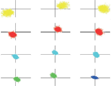
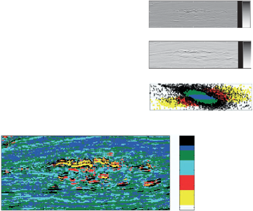
Figure 5.51
Statistical AVO interpretation of a deep sea turbidite reservoir (after Avseth et al.,
2003
): (a) R
0
/G scatter plots generated using the
statistical rock physics database and Monte Carlo simulation, (b) intercept and gradient sections and calibrated AVO plot (note that the
'background'
trend is in black, (c) section showing predicted lithofacies.
(7) Use the probability model to predict boundaries
from seismic (the number of interface categories
can be reduced to reflect pay (oil and gas) vs non-
pay outcomes).
be representative (and upscaled), with several
wells at least needed to condition the model.
Other issues include reflector interference and the
effect of seismic noise, both on the AVO crossplot
(see
Section 5.6
) and in AVO calibration (see
Section 6.3.3
).
Figure 5.51
illustrates some key components of
statistical AVO, including Monte Carlo simulation
of modelled AVO responses and the need to
'
cali-
5.5 Rock properties, AVO reflectivity
and impedance
There are many ways of using AVO for the inter-
pretation of fluid and rock content from seismic.
Perhaps the most important, however, is the use of
brate
the background trend. Whilst accounting for
rock physics variability is a good thing there are
some significant issues that the interpreter would
need to address before accepting the results with
confidence. Assuming that the lithofacies are opti-
mally defined it is clear that the statistics need to
'
92