Geoscience Reference
In-Depth Information
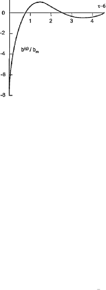
Fig. 15.2.
The magnetic variation
b
(
g
)
/b
m
versus dimensionless time
τ
where
δ
(
t
) is the delta-function,
V
0
and
t
0
are compression-depression ampli-
tude and time-scale, respectively.
Referring the reader to [1] for the actual calculations we present here
the final expression for the magnetic field induced by the plane acoustic
pulse:
b
=
B
0
q
{
α
exp [
−
α
(
τ
−
z
1
)]
−
S
exp [
−
Ω
0
(
τ
−
z
1
])
−
I
(
τ
)
}
,
(15.22)
where
ρ
(0)
ρ
(
z
1
)
1
/
2
ρ
(0)
ρ
(
z
1
)
1
/
2
q
=
ζ
(
z
1
)
lV
0
t
0
ω
2
=
4
πσ
C
(
z
1
)
lc
s
V
0
t
0
z
1
c
2
∗
,
(15.23)
z
1
c
s
1
I
(
τ
)=
k
3
2
π
Ω
{
Ψ
+
(
Ω, τ
)exp(
kz
1
)+
Ψ
−
(
Ω, τ
)exp(
−
kz
1
)
}
dΩ.
(15.24)
−
1
Here
k
2
Ω
2
2
k
sin (
Ωτ
)
Ψ
±
(
Ω, τ
)=
nΩ
cos (
Ωτ
)
−
±
,
2
k
]
2
n
2
Ω
2
+
k
2
[
Ω
2
±
2)
exp
z
1
Ω
0
−
,
Ω
0
4(
Ω
0
−
2
Ω
0
α
=2
/ζ
(
z
1
)
,
S
=
2
Ω
0
=
2
√
2+2
.
n
=
1
4
dη
(
z
1
)
dz
1
,
τ
=
tω
∗
,
Figure 15.2 shows
b
(
g
)
/b
m
as a function of
τ
for
α
=20
,Ω
=2
.
2and
S
=7
.
5
.
The origin corresponds the time
t
≈
6 min when the sound wave
10
4
cm/s coming to the conductive layer. One can see that
the magnetic field reaches the maximal value
b
m
=
B
0
qS
.
with
c
s
=3
.
3
×


Search WWH ::

Custom Search