MHD-Wave Generation by HF-Heating - Hydromagnetic Waves in the Magnetosphere and the Ionosphere - page 370

0.8

O +

1.1 0.7

N * NO +

N

1 0.6

0.9 0.5

N e

N e

N *

0.8 0.4

0.7 0.3

100 150 200 100 110 120 130

Time, s Time, s

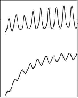
Fig. 13.5. Time variations of normalized ion components for minimum (left) and
maximum solar activity (right) for τ T =10s

• 10 s temperature oscillations yield depths of modulation of N e , an order

of magnitude smaller than in the case of 100 s oscillations.

13.4 Ionospheric Conductivity

We assume that a powerful HF-wave travels through a medium with a new
established value of N e determined by the temperature dependence of the
effective recombination rate. Let
N e = N e 0 1+ γ T e −

T e 0
T e 0

, (13.16)

with the parameter γ is introduced to take into account the dependence of the
N e variations on the modulation period of the HF-wave. For the estimates we
put γ =0 . 5and γ = 1, which correspond roughly to a period at 100 s and to
the quasi-stationary case.
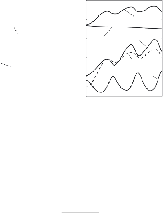
Figure 13.6 shows the relative disturbances of δΣ P (solid and chain lines)
and δΣ H (dashed and dotted lines) determined from a numerical solution of
(13.3) with N e dependent on T e in accordance with (13.16). Here, as well as
in Fig. 13.2, the applied electric field is E = 5 V/m. Comparing Figures 13.2
and 13.6, we see that the displacement of the ionization balance in the pump
wave leads to a growth of the conductivity to 10

− 20% in the daytime and to

50% in the nighttime.
Of course, the self-action of a strong wave, especially in the night
ionosphere, leads to distortion of its modulation. We will not consider these