ULF-Sounding of Magnetosphere and Earth - Hydromagnetic Waves in the Magnetosphere and the Ionosphere - page 333

1.00

k x =410 −3 km −1

k x =10 −3 km −1

0.10

k x =10 −4 km −1

0.01

0.00

0 100 200 300 400 500 600

period[s]

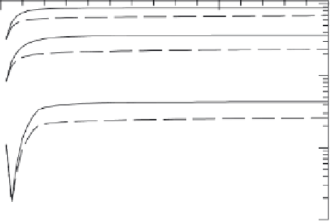
Fig. 11.8. Amplitude of the above-ionosphere field-aligned magnetic component b
versus oscillation period. The curves correspond to three horizontal wavenumbers
and refer to two geoelectric models. The first one is the one-layered one (solid line)
and the second one is the two-layered model (dashed line). In the 1-st model the
resistivity of the 1-st layer is ρ =10 3 Ohm · m and thickness is h 1 = 100 km. In
the two-layered model the resistivity of the upper layer is ρ 1 =10 1 Ohm · m, and
thelowerlayeris ρ 2 =10 3 Ohm · m. Respectively, thicknesses are h 1 = 50 km, and
h 2 = 50 km. The basement is the perfect conductor in the both models

where

ik
k 0

Z ( m )

1 −

g

R g = .

1+ ik

k 0 Z ( m )

g

The angle I is the dip of the magnetic field, Z ( m g is a surface impedance of the
ground, E A is the electric field amplitude of the Alfven wave in the ionosphere
(see (7.136)).
Thus it is possible to get information about the geoelectrical cross-section
by using the properties of waves reflected from the ionosphere. This statement
is correct only if the scale of the initial perturbation will be approximately
equal to or exceed the thickness of the atmosphere h . An attenuation of the
wave is proportional to exp ( kh ). Therefore for a large k the wave loses

information about the surface impedance of the ground.
The dependencies of the longitudinal component b

−

on the period for

10 − 3 km − 1 , are shown in Fig. 11.8
by solid lines for a one-layer model and for a two-layer model (dashed line).
The basis is a perfect conductor in both cases. It can be seen that moving
from one model to another, b is approximately double for small k .

wavenumbers k x =10 − 4 , 10 − 3 and 4 ×