Effective Conductivity of a Cloudy Ionosphere - Hydromagnetic Waves in the Magnetosphere and the Ionosphere - page 309

2.2

2.0

1.8

1.6

1.4

1.2

1.0

2

0 4 6 8 10 12 14 16

β = ω H τ c

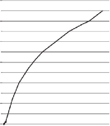
Fig. 10.6. The ratio of effective Pedersen conductivity σ e P to spatial average Ped-
ersen conductivity σ P as a function of the magnetization parameter β e . σ 01 and
σ 02 refer to the local conductivities of inhomogeneities of the 1-st and 2-nd kind,
respectively. The curve with x 1 =0 . 5 relates to the case when areas of the two
components are equal. The curve with x 1 =0 . 1 shows σ e P ( β ) / σ P ( β ) in which
10% of the whole area is occupied by a highly conductive component of σ 1 , whereas
the rest of the mixture is σ 1 =0 . 9 σ 1

The influence of inhomogeneities was defined from the relation of depen-
dency of conductivity on under conditions of non-uniform photoexcitation

σ e xx ( B 0 ) and uniform σ xx ( B ).
Figure 10.6 shows the dependence of σ e P ( β ) /σ P ( β ) on the intensity of the
applied magnetic field. One can see a distinct difference between this and the
dependence of σ eff on the magnetic field. The influence of the conductivity on
|

| B 0 |

B | becomes visible only when β e > 1. In particular, at β = 15 the value of

σ e P ( B ) /σ P ( B ) reaches 2 . 1.

10.4 Discussion

The nature of the anomalous increase of Pedersen conductivity in an
ionosphere with weak fluctuations of electron density, may be explained by
the following process. First, polarization fields originate in inhomogeneous
ionosphere. Next, they produce additional Pedersen and Hall currents whose