Geoscience Reference
In-Depth Information
y
_
+
j
H1
=σ
Η1
E
0
j
x
σ
2
_
+
r=a
j
P1
=
σ
P1
E
0
_
σ
1
+
E
0
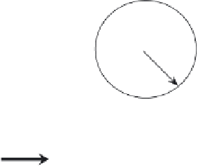
Fig. 10.1.
Isolated inhomogeneity
Alfven and Felthammer demonstrated in one specific example that chang-
ing the local specific conductivity in a plasma slab by 20% compared with the
background specific conductivity, can change the effective conductivity in a
strong magnetic field by an order of magnitude [1].
Local Inhomogeneity Example
The unusual behavior of
σ
eff
in a strong
B
0
can be demonstrated using a
simple example. An isolated cylindrical inhomogeneity of tensor conductivity
σ
2
(
z
) is placed in a medium of
σ
1
(
z
) conductivity. For the sake of simplicity,
we suppose that the external
B
0
is applied along the cylindrical axis
z
and
that the electric field
E
0
is perpendicular to the cylinder. We also assume
that currents do not penetrate from one height level to another. This would
be the situation for two conjugate ionospheres with identical properties. An-
other example is a conductive layer bounded by nonconductive media. Then
the considered example is identical to a circle inhomogeneity with a tensor
conductivity
σ
2
placed on a thin conductive sheet with conductivity
σ
1
(see
Fig. 10.1). A magnetic field
B
0
is perpendicular to the sheet plane. Let the
applied electric field be
E
0
. This electric field produces the dc electric current
j
1
=
j
P
1
+
j
H
1
where
j
P
1
is the Pedersen current and
j
H
1
is the Hall cur-
rent. Let axis
x
the Cartesian coordinate system
with its origin in the
center of the circle and
x
-axis along the current
j
1
=(
j
1
,
0). We also use the
cylindrical coordinate system
{
x, y
}
{
ρ, ϕ
}
. The inhomogeneity causes an anomalous
current
j
(
r, ϕ
)=(
j
r
,j
ϕ
).
The boundary conditions are: continuity of the radial current component
j
r
and of the tangential electric field component
E
ϕ
at
r
=
a
0
. Then
j
r
and
j
ϕ
outside the inhomogeneity are
j
r
j
ϕ
=
j
1
1
+
a
0
r
2
c
cos
ϕ
sin
ϕ
,
−
b
(10.2)
b
c


Search WWH ::

Custom Search