Geoscience Reference
In-Depth Information
1.5
250
500
1
G
m
0.5
1000
σ
g
=10
7
s
−1
1500
0
2000
2500
σ
g
=10
6
s
−1
−0.5
G
m
= (
σ
g
→
•
2000
−1
G
g
1500
1000
σ
g
=10
6
s
−1
−1.5
σ
g
=10
5
s
−1
750
σ
g
=10
5
s
−1
G
g
(σ
g
=10
6
s
−1
)
500
−2
250
−2.5
σ
g
=10
7
s
−1
12
3
−3
0
1000
2000
3000
4000
5000
6000
7000
Distance, km
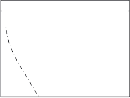
Fig. 8.8.
The amplitude of the magnetic field on the ground as a function of dis-
tance from the point of entry of the incident Alfven wave computed with (8.54)
(solid lines). Dayside ionosphere.
T
= 100 s
.
The ground is a conductive half-space.
σ
g
=10
5
s
−
1
,
10
6
s
−
1
,
10
7
s
−
1
(thin lines) and perfectly conducting (thick line). The
magnetospheric
G
m
and ground
G
g
(8.54) are correspondingly shown by the dotted
and chain lines. The analytical approximation of the magnetic component (8.29)
is the dashed curve. Two curves in the upper right corner show hodographs of the
'ground' and 'magnetospheric' waves versus distance for
T
= 100 s and
σ
g
=10
6
s
−
1
.
Numbers along the curves mark the distance from the source in kilometers. The ra-
dius connect to the origin of the coordinate system and a point on the curves is ln
A.
Here
A
is the amplitude of the horizontal magnetic component of the corresponding
wave mode and angle between the radius and horizontal axis is a phase of the mag-
netic component. Values of
d
g
for
σ
g
=10
5
,
10
6
,
10
7
s
−
1
are marked by asterisks on
the distance axis with numbers 1
,
2
,
3
,
respectively
8.5 Summary
Figure 8.8 shows the amplitude (
A
) of the ground meridional magnetic com-
ponent in the log-scale as a function of distance from the axes of the in-
cident Alfven beam. The magnetic field amplitudes in the beam are given
in the form exp(
x
2
/
2
l
0
). The spatial distributions for different values of
ground conductivity are calculated by (8.54). The integral in (8.54) was cal-
culated with the aid of the Chebyshev-Laguerre quadrature formulae with
the weight coecient numbers 5
−
30 ([1], [9]). Kramp function
w
(
V
m,g
)was
calculated with the method proposed in [8]. For comparison, the curve de-
−
scribed by the analytical expression (8.29) with
L
0
=
√
2
πl
0
is shown in
the same figure by a dashed line. In the calculations, the half-width of the
model source is taken to be equal to
l
0
= 200 km. The oscillation period
is
T
= 100 s
.
The calculations are carried out for the dayside ionospheric
model in the minimum of the solar activity:
Σ
P
=0
.
12
10
9
km/s,
Σ
H
=
×
10
9
km/s. The ground is assumed to be a half space with specific
0
.
14
×


Search WWH ::

Custom Search