Geoscience Reference
In-Depth Information
2.0
1
2.0
a
b
2
1
1.6
1.6
3
2
1.2
1.2
4
0.8
0.8
3
0.4
0.4
4
4
0.0
0.0
1E-6
1E-5
1E-4
1E-3
1E-2
1E-1
1E-6
1E-5
1E-4
1E-3
1E-2
1E-1
k
x
1/km
k
x
1/km
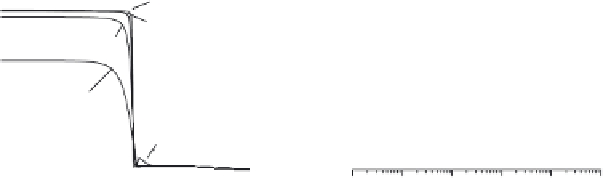
Fig. 7.4.
Comparison of the analytical (by (7.129)) and numerical results for
T
=
10 s (a) and
T
= 100 s (b)
Here integration is extended to the ionospheric region occupied by Hall cur-
rents. We expand the integrand exponent into a series. Then the magnetic
field caused by a height distributed current is equivalent to the field of a thin
current layer located at the altitude
h
=
z
1
σ
H
(
z
1
)
dz
1
σ
H
(
z
1
)
dz
1
.
(7.149)
In another limiting case, the transformation to the thin ionosphere approxi-
mation, as in (7.145), is done directly in the initial equations.
Thus, in problems of ionospheric propagation of low-frequency MHD-
waves, it is possible to use the thin ionosphere approximation for the range of
wavenumbers
10
−
1
km
−
1
.
<L
−
1
|
k
|
≈
7.8 Numerical Examples
Small-Scale Approximation
We begin discussing the results of numerical calculations by estimating the
errors
δR
AA
=
R
AA
−
R
(0)
AA
of approximation (7.129) for various
k
x
,
and
k
y
.
In Figures 7.4a (for
T
= 10 s ) and Fig. 7.4b (for
T
= 100 s) dependencies
of ratio
δR
AA
/R
(0)
AA
on
k
x
are shown for various values of
k
y
. The curve 1
corresponds to
k
y
=10
−
5
km
−
1
, 2 is to 0
.
316
10
−
4
km
−
1
, 3 is to 10
−
4
km
−
1
,
×
10
−
3
km
−
1
. It can be seen that the error in determining
R
AA
by (7.129) is not more than 2% at
T
=10s for
k
x
>
4
and 4 is to 0
.
316
×
10
−
4
km
−
1
and
×
10
−
4
km
−
1
.
Figures 7.5a and 7.5b present amplitude (7.5a) and phase (7.5b) depen-
dencies of
b
3
=
b
sin
I
from
k
x
above the ionosphere (curves 1
,
2) and
b
z
on
the ground (3
,
4) on
k
x
at
k
y
= 0. The curves in Figures 7.5a,b are computed
for the period
T
= 30 s, and in Fig. 7.5c for
T
= 300 s. Curves 2
,
4 corre-
spond to small-scale approximation and curves 1
,
3 correspond to the exact
at
T
= 100 s for
k
x
>
2
×


Search WWH ::

Custom Search