Geoscience Reference
In-Depth Information
2
60
a
Σ
P
=1.55× 10
8
km/s
1,2
b
1
3
50
0
40
1,3
2
2
−
1
30
−
−
−
−
3
1
20
3
3
2
10
1
0
2
4
6
2
4
6
L
−
shell
L
−
shell
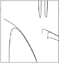
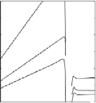
Fig. 6.5.
Half-width of the FLR-shell in the magnetosphere
δ
L
(panel (a)) and its
mapping onto the ionosphere
δ
i
(b) versus the
L−
shell. The curves 1 and 2 at
panel (a) refer to the thin ionosphere and to the I (
L
pp
=4
.
9) and II (
L
pp
=4
.
4)
magnetospheric models, respectively. The 3-rd shows
δ
L
for the thick ionosphere and
I magnetosphere. Curves at (b) refer, respectively, to
Σ
P
=(1
.
55
,
1
,
0
.
5)
×
10
8
km/s
and to the I model
the plasmapause, the cold plasma density falls, and as a consequence of this,
c
Am
increases sharply and the FLR-period is shortened.
An error in
δ
L
caused by the use of (6.104) instead of (6.121) is
∼
0
.
1% at
L<L
pp
and
1% at
L>L
pp
.Atthe
L
corresponding to the plasmapause
location, the error in
δ
L
increases but remains less than 10%. Thus, the ap-
proximate formula (6.104) is valid for calculation of
δ
L
in the whole range
of
L
and will be exploited in further numerical calculations. The half-width
of the resonance region on the ground at the low latitudes is about
δ
i
+
h
(see Chapter 7) and is controlled predominantly by the ionospheric losses.
Equation (6.105) gives
δ
i
≈
∼
200
−
300 km at
L
≈
1
.
5. The height of the high
conductive ionospheric layer
h
≈
100 km.
Close study of the distribution of geomagnetic pulsations at
L
2 could
give information about the boundary of the region where the FLR contributes
mainly to the spatial pulsations' distribution. Note that at low latitudes the
resonance half-width can be found from the observations with the accuracy
of
2 the relative error of
δ
i
obtained from the ground-
based data is essentially higher because
δ
i
itself is about several tens of
kilometers.
The half-width of the FLR-shell in the magnetosphere
δ
L
(frame (a)) and
its mapping onto the ionosphere
δ
i
(frame (b)) as a function of the
L
-shell are
shown in Figures 6.5a and 6.5b. The curves 1 and 2 at frame (a) refer to the
thin ionosphere and to the I (
L
pp
=4
.
9) and II (
L
pp
=4
.
4) magnetospheric
models, respectively. The 3-rd curve represents
δ
L
for the thick ionosphere and
I magnetosphere. The dependencies
δ
i
(
L
) found from (6.105) for the I model
at
Σ
P
=1
.
55
∼
10 km. At
L
10
8
km/s (curves 1, 2, and 3, respectively) are
shown in Fig. 6.5b. The half-width
δ
i
increases monotonously from
10
8
,1
10
8
,0
.
5
×
×
×
10 km
at
L
= 2 to several tens of kilometers closer to
L
pp
and decreases steeply to
≈


Search WWH ::

Custom Search