Hydromagnetic Resonators - Hydromagnetic Waves in the Magnetosphere and the Ionosphere - page 128

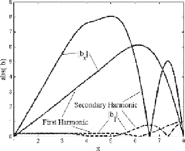
Fig. 5.6. Equatorial distribution of the magnetic field of the first two cavity har-
monics

sum of non-damping normal cavity modes, and in a dissipative medium as
a sum of damping modes. Since a simple enough pattern of the evolution of
plasma perturbations in the hydromagnetic box at k y = 0 was obtained as a
result of rather cumbersome calculations demonstrated in the present chapter,
we shall conclude it with a brief summary of the main results:

• With perturbations along the coordinate y being constant, plasma oscilla-

tions in the box appear as a superposition of non-interacting cavity (FMS)
and Alfven modes.

• In the cavity mode the longitudinal magnetic field and plasma displace-

ment in the direction of the inhomogeneity gradient are finite. Displace-
ment perpendicular to the gradient of the Alfven velocity vanishes, ξ y =0
.

•

In the Alfven mode component ξ y is finite, while b and ξ x vanish.

• The properties of cavity modes in the hydromagnetic box are identical

to the TE mode in an ordinary electrodynamic resonator filled with an
inhomogeneous dielectric. Equation (5.70) is a usual 2D wave equation.
Cavity modes have a discrete spectrum of eigenfrequencies ω k 1 . Arbitrary
perturbation with b and ξ x can be presented as a sum of modes, each of
which changes harmonically in time. With dissipation taken into account,
the harmonics are damped exponentially in time.

• For symmetric harmonics (field-aligned wavenumbers k are odd) (see

Figure 5.7) the transverse electric fields and longitudinal magnetic field
perturbations have an antinode and the transverse magnetic field has a
node in the equatorial plane. For antisymmetric harmonics ( k are even)
the transverse electric fields and longitudinal magnetic field perturbations
have a node, whereas the transverse magnetic field has an antinode in the
equatorial plane.