Geoscience Reference
In-Depth Information
1
100
Phase b
y
|b
y
|
0
0.5
|b
x
|
Phase b
x
100
200
0
5
0
5
5
0
5
x/|δ
1
|
x/|δ
1
|
1
100
Phase b
y
0
|b
y
|
0.5
Phase b
x
100
|b
x
|
200
0
5
0
5
5
0
5
x/|
δ
1
|
x/|
δ
1
|
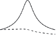
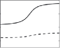
Fig. 5.4.
Amplitude and phase of the magnetic field near the FLR-point. Upper
panels show the results of calculation according to (5.40) at
f
=10
−
2
Hz, normalized
integral Pedersen conductivity
Σ
P
= 10 and Alfven velocity at the resonance point
c
A
= 1500 km/s,
pk
A
=
−
3. The position of the resonance point is at
x
=
x
1
=0
.
Results of numerical integration of (5.7a)-(5.7b) under the same parameters at the
resonance point are shown in the bottom frames
It can be seen from Figure 5.4 that
•
The amplitude of the magnetic field resonance component
b
y
has a peak
of a Lorentz form near the FLR; the phase of
b
y
changes abruptly at
π
when passing the resonance point in the direction of the decrease of the
resonance frequency.
•
Comparison of the upper (according to (5.40) ) and bottom (numerical
integration of (5.7a)-(5.7c)) panels of Fig. 5.4 demonstrates a good agree-
ment of amplitude and phase distribution of the resonance components
b
y
. The behavior of non-resonant components is not so well described by
(5.40). This is due to the fact that the regular part of the solution can be
comparable with its logarithmically singular part.
•
The transversal magnetic field is linearly polarized at the
x
p
point be-
ing displaced at a distance slightly less than the resonance half-width
from the resonance point. In the numerical example
x
p
is displaced to
the right at 0
.
22
|
δ
1
|
.At
x
=
x
p
, the polarization ellipse changes the sign of
rotation.
•
At
x>x
p
the vector rotates counterclockwise when looking along the
z
-
axis and clockwise at
x<x
p
. Thus, the sign of polarization changes near
the maximum and the transversal electric and magnetic fields become
approximately linear in it.


Search WWH ::

Custom Search