Geoscience Reference
In-Depth Information
x
t
x
r
1
2
k
A
1.5
0.8
1
Initial wave
0.6
0.5
0.4
0
c
A
0.2
−
0.5
0
−1
0
5
10
15
20
0
5
10
15
20
x
x
20
x 10
3
4
b
y
/B
0
3
b
||
/B
0
15
2
b
x
/B
0
10
1
5
0
0
−1
−2
5
0
5
10
15
20
0
5
10
15
20
x
x
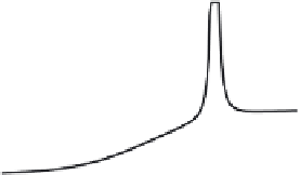
Fig. 4.3.
Left top frame: the Alfven velocity (solid line) and Alfven wave number
(dashed line) as a function of
x
.Righttopframe:Effectivepotential
U
(
x
)
.
The
initial wave propagates from left to right, from the region with low Alfven velocity
to high velocity. Two vertical dotted lines show the location of the turning point
(
x
t
) and resonance point (
x
r
) . Left bottom: wave magnetic field near a resonance
surface. Right bottom: Energy flux to resonance surfaces
it. The incidence of an
H
-polarized wave onto a layered medium has been
considered and solved completely in ([7], [8]).
The qualitative pattern of the fields can be obtained if we wr
ite (4.5
3) in
the form of the Schrodinger wave equation. Substitution
b
=
u
k
A
−
k
2
into
(4.53) gives
d
2
u
(
x
)
dx
2
−
U
(
x
)
u
(
x
)=0
,
(4.54)
where
dk
A
dx
2
d
2
k
A
dx
2
1
2
1
k
A
−
+
3
4
1
k
A
−
U
=
k
y
+
k
2
k
A
−
−
2
.
k
2
k
2
The left top panel of Fig. 4.3 presents the Alfven velocity
c
A
(
x
)and
wavenumber
k
A
(
x
). Dependence of the effective potential
U
(
x
) on the transver-
sal coordinate
x
is shown in the right top panel. The coordinate
x
and
k
A
(
x
)
are normalized on a scale
l
⊥
/
2
.
The function
U
(
x
) is calculated at frequency


Search WWH ::

Custom Search