Optical Imaging - Correction Techniques in Emission Tomography - page 250

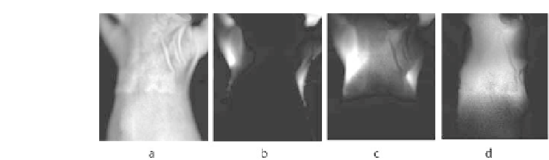
FIGURE 12.5: Measurements of a mouse with fluorescent biodistribution in
the lung. (a) white light image; (b) transillumination excitation light meas-
urement; (c) transillumination fluorescence measurement; (d) normalized flu-
orescence measurement.

measurements. One such approach is termed as the normalized Born approx-
imation [35]. In this method, Equation 12.22 is divided by a measurement at
the emission wavelength:

Z

em (r;r s ;!)
ex (r;r s ;!)

g em (r;r 0 ;!)O f (r 0 ;!) ex
0

(r 0 ; r s ;!)dr 0 =

ex
0

(r 0 ;r s ;!)

(12.19)
where is a constant that accounts for gain factors. This normalization elim-
inates instrumentation-related effects, and reduces the sensitivity of the re-
construction to errors in optical properties. For one source-detector pair the
resulting linear problem formulated in terms of Green's functions is given by

= X G(r 0 ;r s ;!)n(r 0 )G(r;r d ;!)
G(r d ;r s ;!)

em (r d ;r s ;!)
ex (r d ;r s ;!)

dV: (12.20)

The right-hand side is a sum over the voxels into which the imaged volume
V is discretized. The Green's functions G can be computed using analytical
methods [35, 37, 9] or numerical methods [23, 43] such as the Finite Element
Method or Finite Volume Method. G(r 0 ;r s ;!) represents the Green's function
describing light propagating from source position r s to position r inside the
volume, G(r 0 ;r s ;!) describes the light propagating from the point inside the
volume to the detector position r d and G(r d ;r s ;!) is the normalization term.
The volume of the voxels is included by the term dV and n(r 0 ) is the unknown
fluorochrome distribution inside the volume. For the total number of source-
detector pairs N data , the resulting linear problem is written as

y = Wn (12.21)

where y of size 1 N data is the normalized data computed from the meas-
urements at the surface, W of size N data N voxels is called the weight matrix
and n of size 1 N voxels denotes the fluorescent source distribution.