Image Processing Techniques in Emission Tomography - Correction Techniques in Emission Tomography - page 128

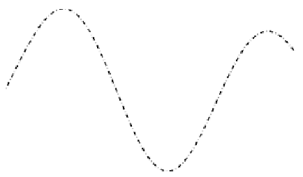
sinc
spline
linear
NN

FIGURE 7.6: Five data points (bold dots) are interpolated with sinc (dash-
dot line), spline (dotted line), linear (dashed line), and nearest neighbor (solid
line) interpolation.

This illustrative one-dimensional example already points out some simi-
larities and differences of different interpolation mechanisms. When choosing
an interpolation method there are different criteria to be considered such as
computation time, differentiability, continuity, and accuracy. Among the pre-
sented methods, nearest neighbor interpolation is the fastest one but it lacks
meaningful derivatives and the results are (in general) not continuous. A dif-
ferentiable and continuous method is spline interpolation, but at the expense
of higher computation costs. Linear interpolation is a compromise as it is rel-
atively fast and continuous. Differentiability is given, except for regular grid
points.
The impact of interpolation is illustrated in Figure 7.7 by scaling up real
PET data. The original image in Figure 7.7(a) shows a human heart. This
image was scaled up by a factor of 20 using NN (Figure 7.7(b)), linear (Fig-
ure 7.7(c)), and spline (Figure 7.7(d)) interpolation. It is obvious that linear
and spline interpolation are superior to NN. The differences between linear
and spline interpolation are not that clear at first glance.

(a) Original (b) NN (c) Linear (d) Spline

FIGURE 7.7: The original image (a) was scaled up using (b) NN, (c) linear,
and (d) spline interpolation.