Quasistatic Poroelasticity - Continuum Mechanics of Anisotropic Materials - page 224

a

dimensionless pressure

1.2
1
0.8
0.6
0.4
0.2

X

0.2 0.4 0.6 0.8 1

− 0.2

b

0.75
0.5
0.2 0

1

pressure

0.8

− 0.25

0.6

0
0.002 0.004 0.006

X

0.4

0.2

τ

0.008

0.01 0

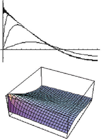
Fig. 8.5 Illustration of the decay of the pressure with time in a layer of poroelastic material resting
on a stiff impermeable base subjected to a constant surface loading. ( a ) The dimensionless pressure
p ( X , t ) /Wp o is plotted (ordinate) against the entire range of the dimensionless layer coordinate
X x 3 / L from 0 to 1 (abscissa) for dimensionless time t values of 0, 0.0001, 0.001, 0.01, 0.1 and 1.

The top curve with the sinusoidal oscillations is the curve for t ¼ 0. The sinusoidal oscillations
arise because only a finite number of terms (200) of the Fourier series were used to determine the
plot. It is important to note that this curve begins at the origin and very rapidly rises to the value 1,
then begins the (numerically oscillating) decay that is easily visible. The curves for values of t of
0.0001, 0.001 and 0.01 are the first, second and third curves below and to the right of the one for
t ¼

¼

0. The curves for values of t of 0.1 and 1 both appear as p ( X , t )/ Wp o ¼ 0 in this plot. ( b ) The

dimensionless pressure p ( X , t )/ Wp o is plotted against the entire range of the dimensionless layer

coordinate X ¼ x 3 / L from 0 to 1 (abscissa) and the range of dimensionless time t from 0 to 0.01

2 p

@ p

c @

o

WP o e i

t

t x 3 ¼

o ;

i

@ @

where the boundary conditions are the same as those in the example above, namely
that p ¼ 0at x 3 ¼ 0 and @ p =@ x 3 ¼ 0at x 3 ¼ L . The solution is obtained by

o

assuming that the pressure p is of the form p

t , thus the partial
differential equation above reduces to an ordinary differential equation,

ð x 3 ; t Þ¼ f ð x 3 Þ

e i