Information Technology Reference
In-Depth Information
and is reproduced from Grigolini
et al
.[
25
]. The solar-flare waiting-time probability
distribution function is determined to be the hyperbolic probability density function
shown in Figure
2.3
. The name waiting time is used because this is how long you wait,
in a statistical sense, before another flare occurs. The data set consists of 7,212 hard-
X-ray-peak flaring-event times obtained from the BATSE/CGRO (Burst and Transient
Source Experiment aboard the Compton Gamma Ray Observatory satellite) solar-flare
catalog list. The data cover a nine-year-long series of events from April 1991 to May
2000. The waiting-time probability distribution of flares is fitted with (
1.41
), where the
stochastic variable
τ
in Figure
2.3
is the time between events. The fit yields the inverse
power-law exponent
05.
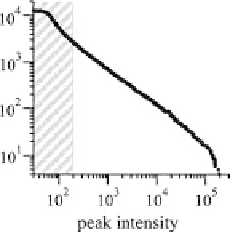
The magnitudes of the solar-flare events themselves are measured in terms of the
number of hard X-rays given off by flares. Figure
2.4
depicts the cumulative distribution
of the peak gamma-ray intensity of solar flares and the relationship is strictly an inverse
power law over nearly three factors of ten when the shaded region is ignored. How-
ever, when the shaped region is included these data can also be fit with the hyperbolic
distribution (
1.41
), but this is not done here. Note the difference between the calendar
time over which the data were recorded which was used to construct the intensity graph
in Figure
2.4
and that used to generate the time-interval distribution in Figure
2.3
.We
expect the underlying mechanisms determining the magnitudes and times of solar-flare
activity to be stable so it is not necessary to have the calendar time of the two data
records coincide. We only require that the sequence of events be sufficiently long that
we have good statistics.
These four examples of event-magnitude and event-time distributions do not show
how the statistics are related to the spatial structure or to the dynamics of the phenomena
being described. The complexity in earthquakes and solar flares is doubly evident in that
both the size and the intervals are hyperbolic distributions. But earthquakes and flares
are probably no more complicated than many other phenomena much closer to home.
In fact it is not necessary to go outside the human body to observe structures that have
the variety of scale so evident in the cosmological distributions. Neurons, for example,
display this variety of scale in both space and time.
β
=
2
.
14
±
0
.
The peak intensity of the gamma-ray spectrum produced by solar flares in counts per second,
measured from Earth orbit between February 1980 and November 1989. Although the data are
taken from the same archive as those used in Figure
2.3
, the time periods used do not coincide
[
53
]. Adapted with permission.
Figure 2.4.