Environmental Engineering Reference
In-Depth Information
(b)
(a)
25
25
20
20
15
15
10
10
5
5
y
= 1.331
x
+ 0.537
R
2
= 0.867
y
= 1.179
x
+ 1.916
R
2
= 0.374
0
02468
Reference wind speed (m/s)
0
02468
Reference wind speed (m/s)
10
12
14
16
10
12
14
16
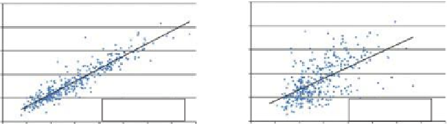
Figure 12-2.
Typical scatter plots of target and reference wind speeds. (a) A relatively high
correlation, indicating that the two sites experience very similar wind climates. (b) A relatively
poor correlation.
Source:
AWS Truepower.
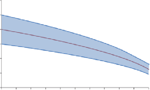
Figure 12-3 plots this equation as a function of
r
2
.One
year of concurrent reference - target data is assumed. Consider the middle curve. When
there is no correlation
for a range of values of
σ
r
2
, the error margin simply equals the annual variability,
in this case 4%. For midrange values of
r
2
, the uncertainty is reduced by one-fourth,
to about 3%. If the correlation is very high, the uncertainty is reduced by nearly 70%,
to 1.3%. As Figure 12-3 suggests, there is usually no point in employing a reference
station with less than a 50%
r
2
value; many resource analysts do not consider stations
with values of
r
2
below 60 - 70%.
An important question is what averaging interval should be applied to the wind
speeds when using the MCP process. The optimal averaging interval for MCP is
(
=
0
)
6.0
5.0
5% Interannual variation
4.0
4%
3.0
3%
2.0
1.0
0.0
0 0 030 0 0 0 0 090
100
Correlation coefficient (
r
2
,%)
Figure 12-3.
The approximate uncertainty margin in the estimated long-term mean wind speed
at a site, assuming 1 year of on-site data and 10 years of reference data, as a function of
the
r
2
coefficient between them and of the interannual wind speed variation
σ
.
Source:
AWS
Truepower.


Search WWH ::

Custom Search