Gravity Changes over Russian River Basins from GRACE - Planetary Exploration and Science: Recent Results and Advances - page 51

3.3 Results of Processing

We applied MSSA in the spectral domain to the Stokes coefficients. The distribution
of singular numbers is represented in Fig. 3.2 . SNs were grouped into several PCs
which were converted into spatial maps of EWH. The first two largest SNs were
grouped into PC 1 capturing annual cycle, the next two SNs into PC 2, representing
trend (slow changes). The sum of MSSA SNs 1-10 represents the largest part of
signal variability (energy). Higher-order PCs (SN >10) contain high-frequency
components, such as noises related to the stripes and some part of the signal from
transient events, such as coseismic deformation after earthquakes. Detailed analysis
of MSSA PCs for global maps was given in Zotov and Shum ( 2009 ).
Simulated Topological Networks (STN-30p, http://www.wsag.unh.edu/Stn-30/
stn-30.html ) database was used to constrain the region of study to the basins of
15 large Russian rivers (Fig. 3.3 , left). Table 3.1 contains information about these
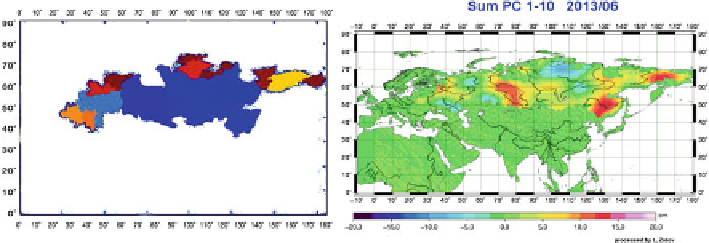
basins. The map of the sum of SNs 1-10 for the last month (06.2013) of the data
span in the constrained area is represented in Fig. 3.3 , right. This map includes
contribution from annual PC 1, long periodic PC 2, and other components except
the stripes, which are mostly removed (they go to SNs >10). The animated maps of
all the obtained PCs are accessible on the website http://lnfm1.sai.msu.ru/~tempus/
GRACE/index.htm .
The signal was averaged over the territory constrained by the basins of 15 large
Russian rivers. Results are shown in Fig. 3.4 . On top the black curve represents the
mean sum of SNs 1-10. The purple curve represents the initial data (sum of all PCs)
before MSSA. It is seen that SNs 1-10 sum includes almost all the variability of
the initial data. The trend (PC 2) is shown in blue. It has a maximum in 2009, then
decreases. This trend is defined mostly by Siberian river basins (Fig. 3.6 ). The red
curve depicts the prediction made in February 2013 by neural network (NN),
containing nine neurons in three layers (Zotov 2005 ). Prediction was made when the
data for spring months were not yet available. Later, when they were obtained, we
found out that the prediction was inappropriate (NN was too simple). The observed

Fig. 3.3 Drainage basins of 15 Russian rivers and the sum of SNs 1-10 over these basins for

06.2013