Geoscience Reference
In-Depth Information
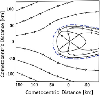
Fig. 10.2
A schematic view
of the Rubin et al. (
2012
)
model of the structure of the
cometary ionosphere of
comet 67P near perihelion
The magnetometer measurements on Giotto (Neubauer et al.
1986
)showed
that the theoretical estimate was nearly correct. Some subsequent first-order one-
dimensional model calculations (Cravens
1986
; Ip and Axford
1987
) demonstrated
that the basic structure of the diamagnetic ionospheric boundary such as the sharp
drop-off of the magnetic field to near zero can be well described by the following
equation (Fig.
10.2
) (Ip and Axford
1987
):
B
R
R
max
D
B
max
Œ1
C
2 ln .R=R
max
/
1=2
ŒR=R
max
(10.3)
If we use Table 6 of comet 67P's gas production rates of H
2
OandCO
2
at different
values of r given in Snodgrass et al. (
2013
) and the pressure balance condition,
B
max
2
/8
mn
sw
v
sw
2
,where
m
is the proton mass and
n
sw
and
v
sw
are, respectively,
the solar wind density and velocity (
400 km s
1
), at
r
with
n
sw
D
5/
r
2
(protons
cm
3
), we can find the size of the diamagnetic ionospheric cavity as a function of r
from the application of Eq.
10.2
.
Figure
10.3
shows that at
r
3 AU where the Rosetta spacecraft is to deliver
the lander,
R
max
10 km. This means that the solar wind should penetrate all the
way to close distances to the comet nucleus according to this simplified treatment.
At perihelion,
R
max
will increase to 35 km. This result is in agreement with MHD
model calculations (Rubin et al.
2012
). Thus, if the Rosetta spacecraft can move
to a cometocentric distance of about 30-50 km, the RPC instrument package will
have the possibility to transverse the critical region where the ionospheric plasma is
decoupled from the neutral gas outflow and be stagnated.
Search WWH ::

Custom Search