Coordinate Systems - Essentials of Interactive Computer Graphics - page 249

Tutorial 10.3. Verify the ± 1 . 0 Drawing Area

Tutorial 10.3.
Project Name
D3D _ ViewTransform2

• Goal. Verify that the application window displays all vertices inside the
range of

± 1 . 0.

• Approach. With all matrix processors set to the identity matrix, draw a
circle with center located at the origin (

( 0 , 0 ) ) and radius of 1 . 0.

Figure 10.4 is a screenshot of running Tutorial 10.3. In this case, the output UI
drawing area is defined to be 200 pixels

200 pixels. Once again, we initialize all
the matrix processors of the D3D API to identity and proceed to draw a unit circle
located at the origin. Recall that we approximate a circle with a triangle fan where
vertices of the triangles are located on the circumference of the circle. We observe
that the circle perfectly fits within the application drawing area.

×

This tutorial

verifies that the reason we need the M w 2 n transform is that the D3D graphics API
automatically transforms all vertices from within the range of
−

Figure 10.4. Tuto-
rial 10.3: Drawing a circle
of radius 1 . 0 and center at
( 0 , 0 ) with D3D

1 . 0 ≤ x ≤ 1 . 0 ,

− 1 . 0 ≤ y ≤ 1 . 0 ,

to the entire application drawing area. In computer graphics, we refer to this Tutorial 10.4.

Project Name
D3D _ ViewTransform3

square area covered by ± 1 as the normalized space, or normalized device coordi-

nate (NDC).

Tutorial 10.5.
Project Name
D3D _ ViewTransform4

Tutorials 10.4 and 10.5. Experimenting with the NDC

• Goal. Understand that the entire NDC is mapped onto the application draw-
ing area, regardless of the dimensions of the application window.

• Approach. Draw the unit circle onto application draw areas with drastically
different dimensions and observe the results.

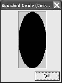
To further understand the transformation performed internally (and automatically)
by D3D, in Tutorials 10.4 and 10.5 we define the UI drawing areas to be 100 pixels
× 100 pixels, respectively. In both tutorials, the

drawing routines are identical to that of Tutorial 10.3, where the same unit circle
with center located at the origin is drawn in each case. Figures 10.5 and 10.6 are
screenshots of running Tutorials 10.4 and 10.5. It is interesting that in both cases,
just as in the case of Tutorial 10.3, the unit circles fit perfectly within the bounds of
the application windows. Of course, in this case, because the application windows
are rectangular, the circles are squashed into corresponding ellipses.

200 pixels and 200 pixels ×

Figure 10.5. Tu-
torial 10.4: Drawing the
same circle onto a 100 ×

200 window.