KINEMATICS - Biomechanics and Motor Control of Human Movement - page 78

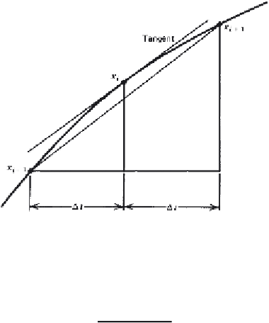
Figure 3.24 Finite-difference technique for calculating the slope of a curve at the i th

sample point.

at the ith sample is:

θ i + 1 − θ i − 1

2 t

ω i = rad/s (3.16)

3.5.4 Accelerations — Linear and Angular
Similarly, the acceleration is:

Vx i + 1 − Vx i − 1

2 t

m/s 2

=

Ax i (3.17)

Note that Equation (3.16) requires displacement data from samples i + 2

and i 2; thus, a total of five successive data points go into the accelera-

tion. An alternative and slightly better calculation of acceleration uses only
three successive data coordinates and utilizes the calculated velocities halfway
between sample times:

−

x i + 1 − x i
t

Vx i + 1 / 2 = m/s (3.18a)

x i − x i − 1

t

Vx i − 1 / 2 = m/s (3.18b)

Substituting these “halfway” velocities into Equation (3.17) we get:

x i + 1 − 2 x i + x i − 1

m/s 2 Ax i = (3.18c)

t 2

For angular accelerations merely replace displacement data with angular data
in Equations (3.17) or (3.18).