KINEMATICS - Biomechanics and Motor Control of Human Movement - page 70

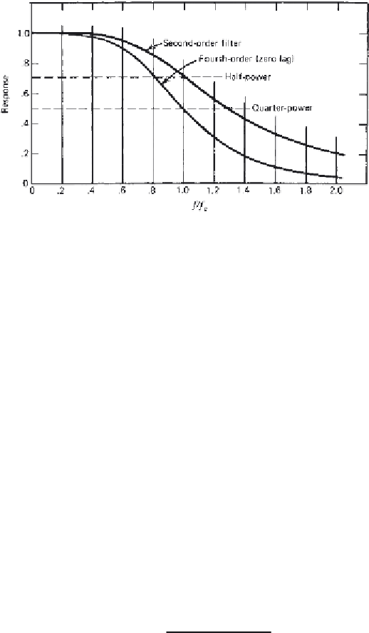
Figure 3.18 Response of a second-order low-pass digital filter. Curve is normalized
at 1.0 at the cutoff frequency, fc. Because of the phase lag characteristics of the filter, a
second refiltering is done in the reverse direction in time, which results in a fourth-order
zero-lag filter.

finite differences from the filtered data, is plotted in Figure 3.19. Note how
repetitive the filtered acceleration is and how it passes through the “middle”
of the noisy curve, as calculated using the unfiltered data. Also, note that
there is no phase lag in these filtered data because of the dual forward and
reverse filtering processes.

3.4.4.3 Choice of Cutoff Frequency — Residual Analysis. There are sev-
eral ways to choose the best cutoff frequency. The first is to carry out a
harmonic analysis as depicted in Figure 3.16. By analyzing the power in
each of the components, a decision can be made as to how much power to
accept and how much to reject. However, such a decision assumes that the
filter is ideal and has an infinitely sharp cutoff. A better method is to do a
residual analysis of the difference between filtered and unfiltered signals over
a wide range of cutoff frequencies (Wells and Winter, 1980). In this way, the
characteristics of the filter in the transition region are reflected in the decision
process. Figure 3.20 shows a theoretical plot of residual versus frequency.
The residual at any cutoff frequency is calculated as follows [see Equation
(3.9)] for a signal of N sample points in time:

N

1
N

X i ) 2

R(f c ) = (X i − (3.9)

i = 1

where f c = is the cutoff frequency of the fourth-order dual-pass filter.

X i = is raw data at i th sample.

X i

= is filtered data at the i th sample using a fourth-order zero-lag

filter.