SIGNAL PROCESSING - Biomechanics and Motor Control of Human Movement - page 16

y

x

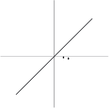
Figure 2.2 Scatter diagram showing a positive correlation between variable x and

variable y .

will be ve in quadrants 1 and 3 and - ve in quadrants 2 and 4, and provided

there are enough points their sum, r, will tend towards zero, indicating no
relationship between the two variables.
Now if the variables are related and tend to increase and decrease together
( x i − x ) and ( y i − y ) will fall along a line with a positive slope in the x - y
plane (see Figure 2.2). When we sum the products in Equation (2.1), we will
get a finite + ve sum, and when this sum is divided by N , we remove the
influence of the number of data points. This product will have the units of the
product of the two variables, and its magnitude will also be scaled by those
units. To remove those two factors, we divide by s x s y , which normalizes the
correlation coefficient so that it is dimensionless and lies between

+

1.
There is an estimation error in the correlation coefficient if we have a
finite number of data points, therefore, the level of significance will increase
or decrease with the number of data points. Any standard statistics textbook
includes a table of significance for the coefficient r , reflecting the error in
estimation.

− 1 and +

2.1.2 Formulae for Auto- and Cross-Correlation Coefficients
The auto- and cross-correlation coefficient is simply the Pearson product
moment correlation calculated on two time series of data rather than on
individual measures of data. Autocorrelation, as the name suggests, involves
correlating a time series with itself. Cross-correlation, on the other hand, cor-
relates two independent time series. The major difference is that a correlation
of time series data does not yield a single correlation coefficient but rather
a whole series of correlation values. This series of values is achieved by