Biomedical Engineering Reference
In-Depth Information
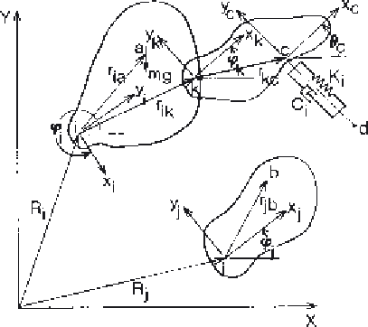
Figure 8.3
Link-segment diagram showing planar modeling of three segments and a
spring damper. Three local references systems are shown. See the text for details.
The velocity vector of the same point is obtained by taking the time deriva-
tive of Equation (8.16). Remembering that
ω
z
=
d θ
z
/dt
,
[
φ
]
˜
ω
r
ia
V
a
=
V
i
+
[
φ
]
v
ia
+
(8.17)
where [
2 skew symmetric angular velocity matrix generated from
the angular velocity vector,
ω
]isa2
˜
×
0
˜
ω
=
−
ω
z
(8.18)
ω
z
0
Now let us return to the sliding block example (see Figure 8.2). Setting
θ
=
45
◦
, then
c
=
cos
(
45
)
=
sin
(
45
)
=
0
.
707, and
ω
=
0. The displacement
and velocity lists are:
[
q
1
,0]
VELO
(
1
)
=
q
1
,0
DISP
(
1
)
=
(8.12
d
)
Since the origin of LRS(1) is
pt(
1
)
, then, from Equation (8.16),
q
2
q
3
]
t
=
[
q
1
+
0
.
707
(d
1
−
q
2
)
−
0
.
707
q
3
,0
.
707
(d
1
−
q
2
)
+
0
.
707
q
3
]
VELO
(
2
)
=
˙
DISP
(
2
)
=
DISP
(
1
)
+
[
φ
][
d
1
−
q
2
)
q
1
−
0
.
707
(
˙
q
2
+˙
q
3
)
,0
.
707
(
˙
q
3
−˙
(8.12
e
)


Search WWH ::

Custom Search