SYNTHESIS OF HUMAN MOVEMENT—FORWARD SOLUTIONS - Biomechanics and Motor Control of Human Movement - page 205

8.2.1 Lagrange's Equations of Motion
The following lines are a brief description of Lagrange's equations of motion
of the second type. The derivation of these equations can be found in any
advanced classical dynamics textbook, such as Greenwood (1977) or Wells
(1967).

8.2.2 The Generalized Coordinates and Degrees of Freedom
One of the first things to be determined in a given system is the number of
coordinates that represent the model. It is important to realize that any set
of time-dependent parameters that give an unambiguous representation of the
system configuration will serve as system coordinates. These parameters are
known as generalized coordinates, and for the sake of generality, they are
denoted by [ q ] t ,

[ q ] t = [ q 1 , q 2 , ... , q n ] (8.1)

The symbol [] t is used to indicate the transpose of an array or a matrix. For
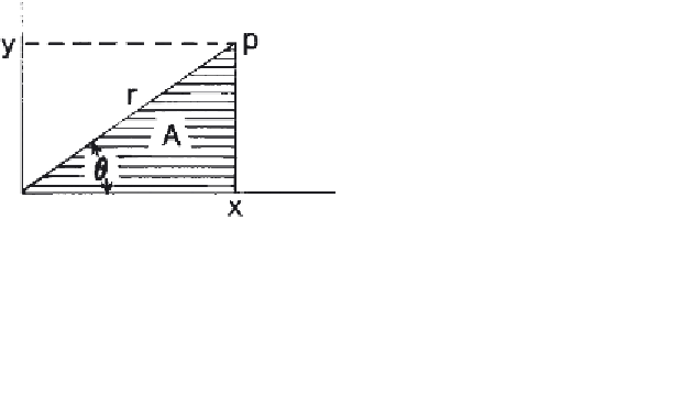
example, consider the particle p in the plane xy , as shown in Figure 8.1. The
point p may be located by several pairs of quantities, such as (x , y) , (r , θ) ,
(A ,sin θ) , (r ,sin θ) , and so on. There is, in fact, no limit to the number of
different coordinate systems that can be defined, which could be used to
indicate the position. Furthermore, the relations between these pairs can be
found easily. Using the first and last pairs, and letting q 1 =

r and q 2 = sin θ ,

(q 2 ) 2 ] 0 . 5

it can be proven that x q 1 q 2 .

A spatial segment can have as many as six degrees of freedom (DOF) (i.e.,
possible coordinates), while a point mass has a maximum of three DOF. A
system degrees of freedom is defined as the sum of the degrees of freedom
of its elements. The degrees of freedom of a system consisting of segments,
S , particles, P , and constraints, C , is given by:

= q 1 [1 − and y =

DOF = 6 S + 3 P − C (8.2)

Figure 8.1 Point p whose position can be specified as a function of several other
variables: r , x , y , θ ,and A .