Graphics Reference
In-Depth Information
In fact, if the representation (10.75) was obtained by substituting the series u(t) in
(10.73) for t in (10.74), then (up to equivalence) all the other different representation
can be obtained by substituting u(wt) for t in (10.74), where w is an arbitrary mth root
of unity. The point a
0
is called a point of
order
m. If m = 1, then a
0
is called a
regular
point. It follows that we are either at a regular point or our surface looks like
wz
m
1
=
.
This finishes our quick look at analytic continuation and Riemann surfaces and
how they play a role in the analysis of complex functions and their singularities. To
keep things as simple as possible we only dealt with holomorphic functions, but in
any serious discussion one would also consider meromorphic functions so that quo-
tients of power series would replace the power series in the discussion above. This
will show up later on when we use quotient fields rather than rings.
We now move on to an example that brings out the relevance of what was just
discussed to algebraic geometry. Consider the affine plane curve
C
in
C
2
defined by
2
2
=-
(
)
.
yx x
(10.76)
Note:
It turns out that for every irreducible cubic curve with an ordinary double
point we can find an affine coordinate system so that in that coordinate system the
curve is defined by the equation (10.76) (see [BriK81]).
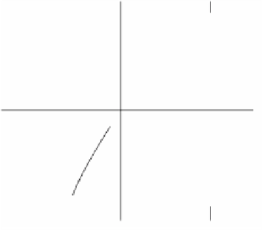
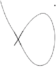
The curve
C
has a singularity at the origin, namely, a double point. See Figure
10.15. We can parameterize the curve by computing the intersection of the lines y =
xt with the curve. This will give the parameterization
()
=
(
() ()
)
ct
xt yt
,
,
where
()
=-
()
=-
2
xt
1
t
3
.
yt
t t
s
+1
r
p¢
r¢
1
s¢
q¢
q
-1
p
Parameterizing y
2
=
x
2
(1
-
x).
Figure 10.15.