Graphics Reference
In-Depth Information
reading that section. What we are doing here is comparing the length of arcs of the
curve with the length its Gauss map “traces out” in
S
1
. If the polygonal curve were an
approximation of a smooth one, then one would be able to show that the polygonal
curvature approximated the smooth curvature defined earlier. See [Call86].
9.4
The Geometry of Space Curves
Next, we consider curves in
R
3
. Such curves are also called
space curves
. Let
[
]
Æ
R
3
FL
:
0
be a parameterization of one of these curves.
Definition.
If F(s) is the arc-length parameterization and T(s) = F¢(s), then the
cur-
vature vector
K(s) and the
curvature
k(s) to the curve F at the point F(s) are defined
by
()
=
()
()
=
()
Ks
T s
and
k s
Ks
.
Note that there is no definition of a signed curvature for space curves. Space
curves are only assigned a nonnegative curvature function.
A geometric definition of the curvature of a space curve:
The approach is again
via best matching circles, but there is more to show now. Given an arbitrary para-
meterization F(t), define circles
C
(t
1
,t
2
,t
3
) through F(t
i
) as before. These circles may
now lie in different planes. Fortunately, one can show that if F≤(t) π 0, then, as the t
i
approach t, the planes determined by the F(t
i
) approach the plane generated by F(t)
and F≤(t) in the limit. Furthermore, the circles
C
(t
1
,t
2
,t
3
) approach a limiting circle
C
that lies in this plane. The curvature at F(t) is then the reciprocal of the radius of this
circle. The C
•
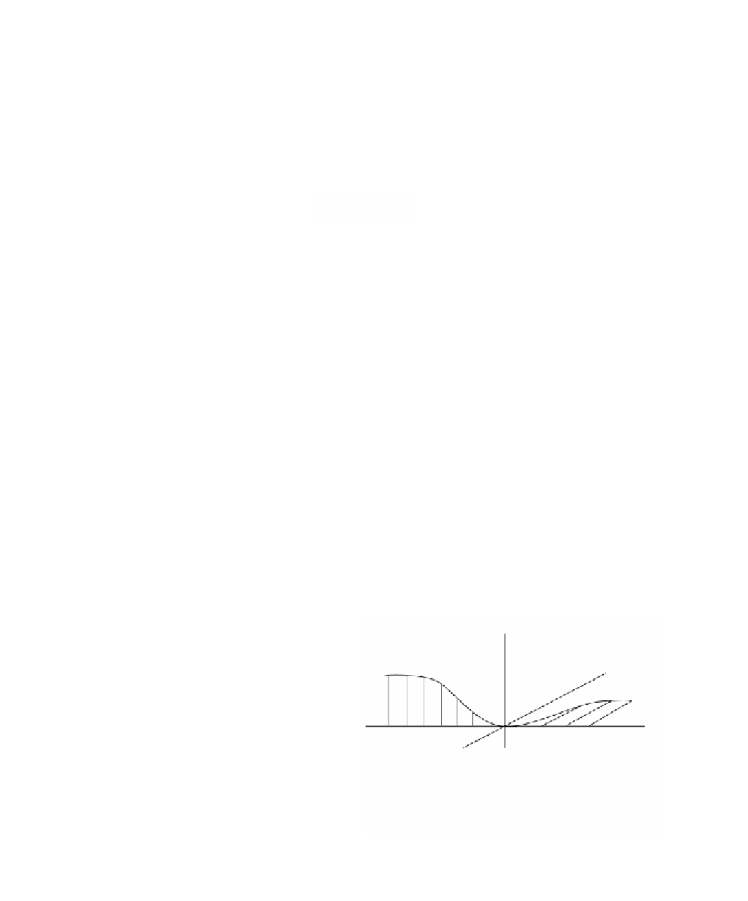
parameterization F(t) in Figure 9.7 shows that the hypothesis F≤(t) π 0
is needed because otherwise there might not be any limiting plane or circle.
z
y
x
F(t) = (0,0,0)
= (t,exp(-1/t
2
,0) , t > 0
= (t,0,exp(-1/t
2
) , t < 0
, t = 0
Figure 9.7.
Why F
≤
(t)
π
0 is needed for a
unique best matching circle.