Graphics Reference
In-Depth Information
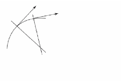
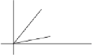
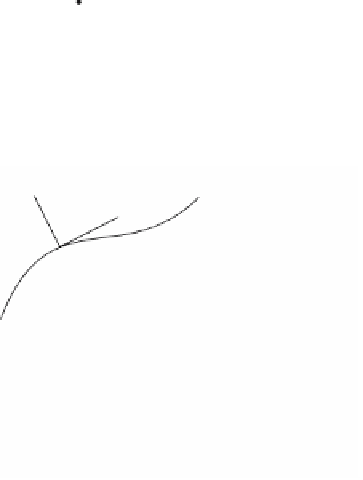
Figure 9.4.
Curvature in terms of rotating
tangent vector.
F¢(t
1
)
F¢(t
2
)
F(t
2
)
F(t
1
)
c
2
F¢(t
1
)
q
F¢(t
2
)
N(s)
T(s)
F(s)
y
N(s)
S
1
F(s)
N(s)
x
1
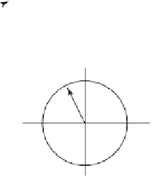
Figure 9.5.
The Gauss map for planar curves.
Let
c
2
be the point that is the intersection of the normal lines to the curve at F(t
1
) and
F(t
2
). One can show that the points
c
2
converge to the center of curvature of the curve
at F(t
1
) and that the expression (9.4) is the reciprocal of the radius of curvature.
In the next part of the discussion it is convenient to switch to arc-length para-
meterization. Let F(s) be the arc-length parameterization of our curve and let T(s) =
F¢(s). There are precisely two
unit
vectors at F(s) that are normal to T(s) at F(s). Let
N(s) denote the one such that (T(s),N(s)) induces the standard orientation of
R
2
. This
defines N(s) uniquely. In fact, since T(s) is a unit vector, if T(s) = (T
1
(s),T
2
(s)), then
N(s) = (-T
2
(s),T
1
(s)).
Now both T(s) and N(s) can be thought of as maps that map the point F(s) on the
curve into the unit circle
S
1
. Thought of in this way, the map N(s) is a special case of
what is called the
Gauss map
whose generalization to surfaces plays a fundamental
role in the study of surfaces. See Figure 9.5. In our second geometric definition of
curvature we could have replace the angle between tangent vectors by the angle
between the corresponding normal vectors since they are the same. The Gauss map
shows that circles naturally come into the picture when studying curvature. Basically,
N(s) relates changes of angles on the curve with the corresponding changes for the
mapped curve in the circle.
With this intuitive introduction to curvature we are ready to give a rigorous def-
inition. The definition is surprisingly quite simple and determining the curvature of