Graphics Reference
In-Depth Information
v
2
b(v
0
v
1
v
2
)
v
2
b(v
1
v
2
)
b(v
0
v
2
)
v
1
v
0
v
1
v
0
b(v
0
v
1
)
sd (K)
K
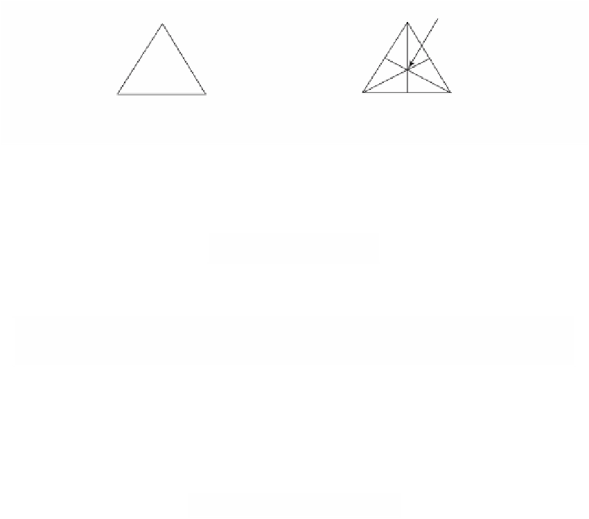
Figure 7.7.
A barycentric subdivision.
Associated to barycentric subdivisions are natural homomorphisms
()
Æ
(
()
)
sd
:
C
K
C
sd K
#
q
q
q
that correspond to sending an oriented simplex [s] to the sum of the oriented sim-
plices into which the barycentric subdivision divides s. For example,
(
[
]
)
=
[
(
)
(
)
]
+
[
(
) (
)
]
+
[
(
)
(
)
]
sd
v vv
b
v vv v
b
v v
b
v vv
b
v v v
b
v vv v
b
vv
#2
012
012 0
01
012
01 1
012 1
12
[
(
) (
)
]
+
[
(
)
(
)
]
+
[
(
) (
)
]
+
b
vvv
b
vv v
b
vvv v
b
vv
b
vvv
b
vv v
0 2 0
.
012
12 2
012 2
0 2
012
See Figure 7.7. More precisely, define the maps sd
#q
inductively on the oriented
simplices as follows:
(1) If
v
is a vertex of K, then sd
#0
(
v
) =
v
.
(2) Assume 0 < q < dim K and sd
#q-1
has been defined. If [s] is an oriented q-
simplex of K, then
[
()
=
()
(
[
()
)
sd
s
b
s
sd
-1
∂
s
.
#
q
#
q
q
(We are using the expression
w
[
v
0
v
1
...
v
q
] to denote the oriented simplex
[
wv
0
v
1
...
v
q
] and let this operation distribute over sums.)
If q < 0 or dim K < q, then we define sd
#q
to be the zero map.
7.2.2.9. Lemma.
The maps sd
#q
are well-defined homomorphisms. Furthermore,
∂
q
°
sd
#q
= sd
#q-1
°
∂
q
, so that sd
#
= (..., sd
#-1
,sd
#0
,sd
#1
, . . .) is a chain map that induces
homomorphisms
()
Æ
(
()
)
sd
:
H
K
H
sd K
.
q
q
q
*
Proof.
This is an easy exercise. See [AgoM76].
We can extend our definitions and define homomorphisms
(
)
n
()
Æ
n
()
sd
:
C
K
C
sd
K
q
q
#
q