Graphics Reference
In-Depth Information
(
()
)
=
Ú
Ú
Ú
()
()
vol T
A
1
=
det
T
¢ =
det
T
¢
1
=
det
T vol
A
.
T
(
A
)
A
(
)
T
A
A
A
Note.
Some, but not all, proofs of Theorem 4.8.6, like the one given by Spivak
([Spiv65]), rely on having proved Corollary 4.8.8 as a special case when
A
is an open
rectangle, so that the corollary would have to be proved separately. This is not hard
to do. One can prove Corollary 4.8.8 by choosing some very simple linear transfor-
mations for which the result is trivial to prove and which have the property that any
linear transformation is a composite of them. See [Spiv65].
Definition.
Let
p
,
v
1
,
v
2
,...,
v
k
Œ
R
n
. Assume that the vectors
v
i
are linearly inde-
pendent. The set
X
in
R
n
defined by
k
Ó
˛
Â
a
Xp
=+
v
0
££
a
1
ii
i
i
=
1
is called a
parallelotope
or
parallelopiped
based at
p
and spanned by the
v
i
. If the ref-
erence to
p
is omitted, then it is assumed that
p
is
0
. If k = 2, then
X
is also called a
parallelogram
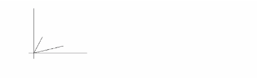
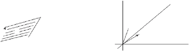
. See Figure 4.26.
Let
X
be a parallelotope in
R
n
4.8.9. Corollary.
based at
p
and spanned by some
vectors
v
1
,
v
2
,...,
v
n
. Then
v
v
Ê
ˆ
1
Á
Á
Á
˜
˜
˜
2
M
()
=
vol
X
det
.
Ë
¯
v
n
Proof.
Because translation does not change volume, we may assume that
p
=
0
.
Define a linear transformation T :
R
n
Æ
R
n
by T(
e
i
) =
v
i
. Clearly, T maps the unit cube,
that is, the parallelotope based at
0
and spanned by
e
1
,
e
2
,...,
e
n
, to
X
. Since the
volume of the interior of the parallelotope is the same as the volume of the paral-
lelotope, the result now follows from Corollary 4.8.8.
y
z
y
v
3
v
2
X
X
v
2
v
1
v
1
x
x
(b) parallelotope in R
3
(a) parallelogram in R
2
Figure 4.26.
Parallelotopes
X
at the origin.