Graphics Reference
In-Depth Information
for some C
•
functions h
ij
. Hence
n
Â
(
)
=
(
)
f x
,
x
,...,
x
x x h
x
,
x
,...,
x
.
12
n
i
j
ij
12
n
ij
,
=
1
By replacing h
ij
by (1/2)(h
ij
+ h
ji
), if necessary, we may assume that h
ij
= h
ji
in some
neighborhood of
0
. Furthermore, the matrix (h
ij
(
0
)) is just the Hessian matrix of f.
Since this matrix is assumed to be nonsingular, we can copy the diagonalization proof
for quadratic forms given in Theorem 1.9.11 (see also [Miln63]) to finish the result.
4.6.4. Corollary.
Nondegenerate critical points of functions are isolated.
The Morse Lemma and its corollary show that one has a good understanding of
what the graph of functions look like near a nondegenerate critical point. The situa-
tion is much more complicated in the degenerate case.
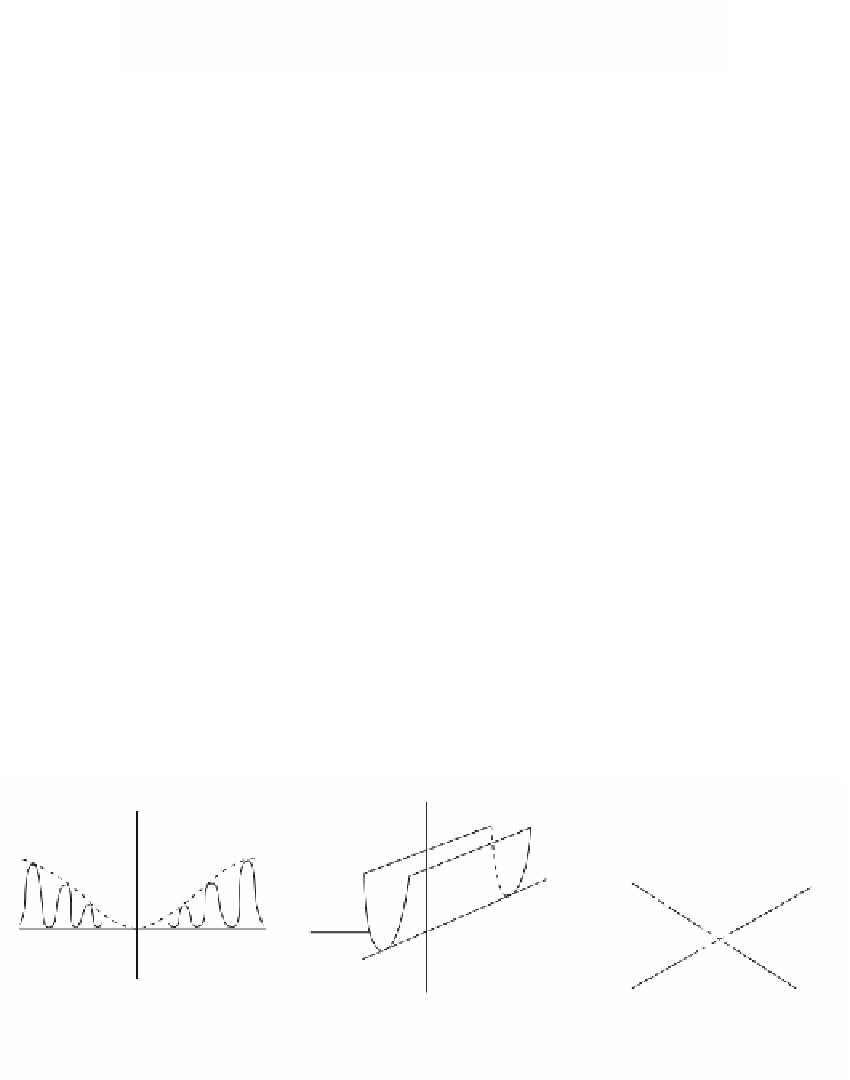
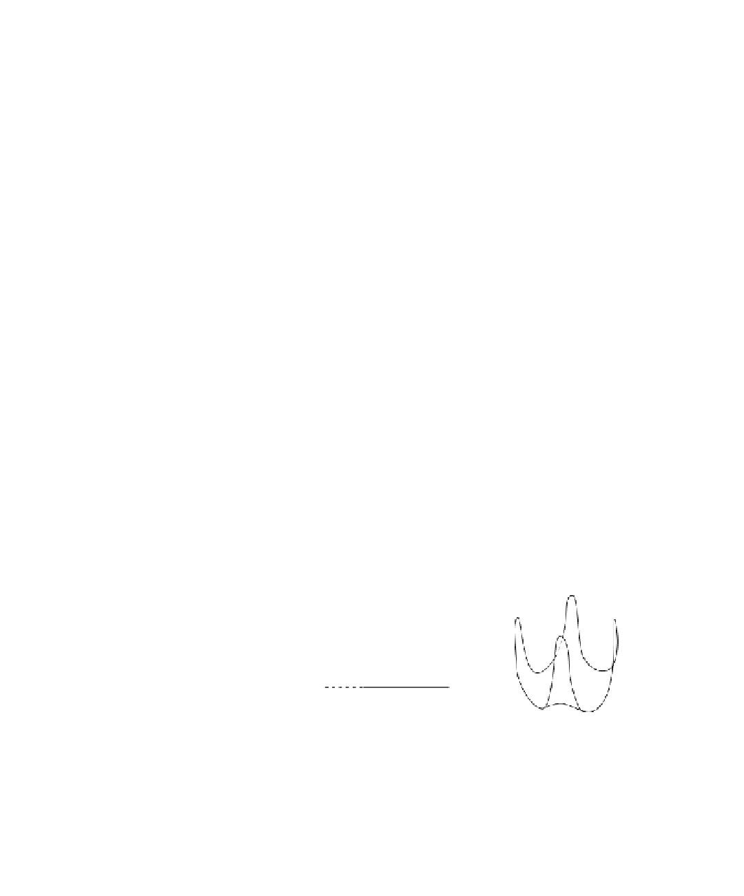
4.6.5. Example.
Consider the functions
(1) f(x) = e
-1/x
2
sin
2
(1/x)
(Figure 4.18(a))
(2) f(x,y) = x
2
(Figure 4.18(b))
(3) f(x,y) = x
2
y
2
(Figure 4.18(c))
All these functions have the origin as a nonisolated degenerate critical point. The func-
tion in (1) has a sequence of nondegenerate critical points converging to the origin.
All the points on the y-axis are degenerate critical points for the function in (2). All
the points on both the x- and y-axis are degenerate critical points of the function in
(3).
We shall see later in Chapter 8 that one can tell a lot about the topology of a space
from the nondegenerate critical points of functions defined on them.
z
y
y
x
x
f(x) = e
-1/x
2
sin
2
(1/x)
f(x,y) = x
2
f(x,y) = x
2
y
2
(a)
(b)
(c)
Figure 4.18.
Examples of nonisolated degenerate critical points.