Graphics Reference
In-Depth Information
Proof.
The Taylor expansion for functions of two variables can be used to prove (1)
and (2). See [Buck78]. It is easy to check that the functions in Figure 4.13(a) and (b)
fall into case (1) and that the function in Figure 4.13(c) (equation (4.13)) falls into
case (2). To prove (3), consider the functions
(a) f(x,y) = x
4
+ y
4
(b) g(x,y) =-(x
4
+ y
4
)
(c) h(x,y) = x
2
- 5xy
2
+ 4y
4
= (x - y
2
)(x - 4y
2
)
Each of these functions has D = 0. The function f has a minimum at (0,0) and g has
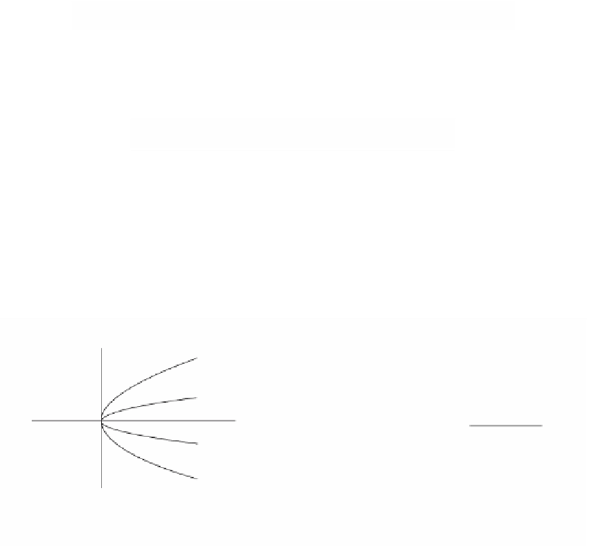
a maximum at (0,0). The function h has a saddle point at (0,0). See Figure 4.14(a).
The “+” and “-” in the figure indicate the regions where the function is strictly posi-
tive or strictly negative, respectively. On the other hand, note that h(x,y) has a local
minimum along any line through the origin. To see this, define
(
)
(
)
=-
()
=
(
)
=-
22
22
2
23
44
s x
h x mx
,
x
m x
x
-
4
m x
x
5
m x
+
4
m x
.
The function s(x) describes h(x,y) along the line y = mx. A direct computation shows
that s¢(0) = 0 and s≤(0) = 2, proving the claim. Along the y-axis we have that h(0,y) = 4y
4
,
and so we also have a local minimum at 0. This finishes the proof of Theorem 4.5.4,
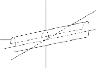
but before we move on, consider another interesting function that has D = 0, namely,
2
(
)
=-
2
2
(
)
k x y
,
1
x
+
4
xy
-
4
y
=- -
1
x
2
y
.
See Figure 4.14(b). Here we have a function that is constant along every line of the
form x - 2y = c. Every point on the line x - 2y = 0 is a critical point.
As in the case of functions of one variable, there is more to finding relative extrema
of functions of two variables than just Theorem 4.5.4. We must always check the func-
tion on the boundary of its domain separately. This basically reduces to finding the
relative extrema of a function of one variable, a problem we have already handled.
z
y
y
x = y
2
+
+
-
x = 4y
2
1
x = 2y
+
+
x
x
-
+
+
h(x,y) = (x - y
2
)(x - 4y
2
)
k(x,y) = 1 - (x -2y)
2
(a)
(b)
Figure 4.14.
Case (3) of Theorem 4.5.4.