Geology Reference
In-Depth Information
the histograms, or redistributing the DNs following some
speci
c function, such as a Gaussian distribution. More
complicated stretches involve giving one part of the dis-
tribution more weight than other parts in order to empha-
size detail.
Filters. Filtering involves manipulating multiple pixels
as sets within the image. For example, boxcar
filters give a
weighted value to each pixel as a function of the value of its
neighbors (the
“
box
”
), which is then slid across the image,
adjusting each pixel one-by-one. In a low-pass
filter the
value of the central pixel is the average value of the neigh-
boring pixels, and the image tends to be smoothed, enhanc-
ing broad changes in the scene (
Fig. 2.15(c)
); the larger the
boxcar, the smoother the result.
In high-pass
filters the DN values from the low-pass
filter are subtracted from the image, leaving only the
smaller variations in the scene and producing a somewhat
sharper image (
Fig. 2.15(d)
). Edge-enhancement
filters
decrease the contrast where pixels have similar values and
enhance the contrast where pixels change, in order to
emphasize the boundaries in the scene (
Fig. 2.15(e)
).
Common
“
snapshot
”
digital cameras automatically
apply some form of stretching and
filtering to produce
pleasing images. Once in the computer, stretching,
filter-
ing, and various color-enhancement
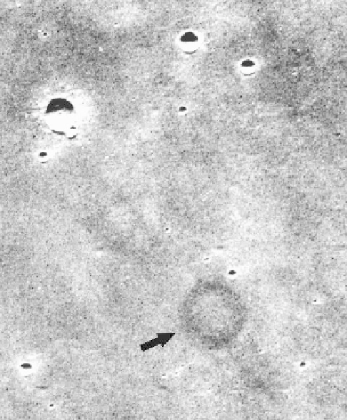
Figure 2.16.
are image blemishes (arrow) caused by dust
grains in camera systems. These and other artifacts can be removed
in image processing by mapping the pixels that are affected and
then assigning DN values to them on the basis of the values of the
surrounding unaffected pixels. This represents cosmetic processing
and users need to be aware that the assigned pixel values are
arti
cial (NASA Viking Orbiter 826A68).
“
Donuts
”
techniques are
applied with user-friendly
“
black box
”
programs that are
based on the processes outlined above.
Geometric projections. In most spacecraft images, the
position of each pixel is referenced to some system, such
as geographic coordinates by latitude and longitude. This
allows the image to be re-cast into standard projections.
For example, an image might be taken that is oblique,or
viewed looking at the terrain at an angle similar to the
view from an airplane window. Because the geometric
position of each pixel is known, they can be shifted so
that the image is portrayed orthographically as though it
were taken as viewed looking straight down on the terrain
(
Fig. 2.17
). Alternatively, the image can be re-projected
into a standard cartographic product, such as a Mercator
projection, depending on the intended use.
Mosaics. Multiple frames can be put together as
mosaics (
Fig. 2.18
), in which the boundaries between
individual frames are seamless. This begins with the iden-
ti
cation of individual tie points that consist of speci
c
features, such as small craters, that are visible on more
than one frame. The pixels in the frames are then re-
projected geometrically so that all of the features match.
Various
filters are then applied so that the pixel DN values
along the frame boundaries are averaged to reduce the
that particular camera so that, when images are subsequently
taken, they can be calibrated or adjusted pixel-by-pixel.
Despite the best efforts to maintain cleanliness, dust
grains
find their way into imaging systems and can pro-
duce artifacts, such as
“
donuts
”
(
Fig. 2.16
). As part of the
calibration routine, these and other artifacts are mapped so
that they can be taken into account and cosmetically
corrected, as noted below.
Calibrations are also typically performed during
ight
because detectors can change with time. Such calibrations
are accomplished by taking images of known surfaces, such
as the Moon or star
fields, with individual pixels adjusted,
just as is done in pre-
ight calibrations. New artifacts can
also occur, as when cosmic rays
“
zap
”
the detector and
degrade or knock out one or more pixels. These artifacts
are also mapped and can be corrected cosmetically.
Stretches. Stretching digital images involves shifting
the distribution of DN levels (
Figs. 2.15(a)
and
(b)
), or
bringing about a simple increase in brightness by moving
all the DNs to a higher level without changing the shape of