Modeling and Nonlinear Analysis in fMRI via Statistical Learning - Advance Image Processing in Magnetic Resonance Imaging - page 556

+ e

Support vectors

0
− e

d

d

− e + e

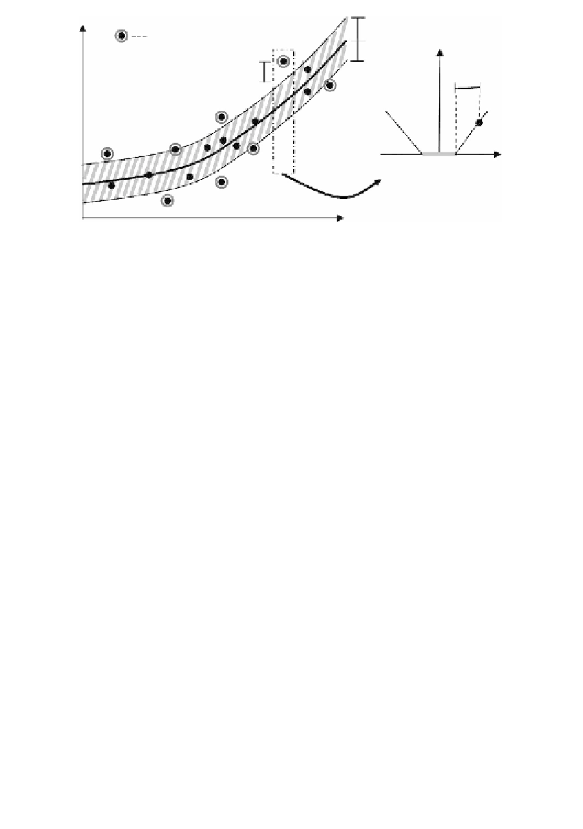
FIGURE 18.2 Diagram of SVR, showing the ε -insensitivity region (shaded area) and the

support vectors.

Only the points outside the shaded region contribute to the cost, and the
deviations are penalized in a linear fashion.

in Equation 18.4 is the trade-off
constant between the smoothness of the SVR function and the total training error.
When the approximation function cannot be linearly regressed, the kernel function
maps training examples from the input space to a high-dimensional feature
space

C

between the output
and the mapped input data points can now be linearly regressed in the feature
space.

ℑ by x → ℑ Φ () x , in such a way that the function f

K describes the inner product in the feature space:

Kx x (, ) = ΦΦ () ( ) x x (18.5)

i j i j

There are different types of kernel functions. A commonly used kernel func-
tion is the Gaussian radial basis function (RBF):

−− || xx ||

2

i j

Kx x (, ) exp = (18.6)

i j

2 σ

2

Maximizing the SVR objective function in Equation 18.2 by SVR training
provides us with an optimum set of Lagrange multipliers α , ∀∈ i [, 1 M ] . The

i

of the estimated SVR function in Equation 18.1 can be computed
by adjusting the bias to pass through one of the given training examples with
nonzero

coefficient b

.
With the nonlinear kernel mapping, the regression function in Equation 18.1
can be interpreted as a linear combination of the input data in the feature space.
Only those input elements with nonzero Lagrange multipliers contribute to the
determination of the function. In fact, most of the

α

i

α 's are zero. The training data

i

with nonzero α are called support vectors , which are the data points not inside

i

the ε -insensitivity region as shown in Figure 18.2. Support vectors form a sparse