Modeling and Nonlinear Analysis in fMRI via Statistical Learning - Advance Image Processing in Magnetic Resonance Imaging - page 555

x 2 z 3

Input data space
ℜ

Feature space
ℜ

2 3

Φ

x 1

z 1

z 2

Left: nonlinear classifier Right: linear classifier

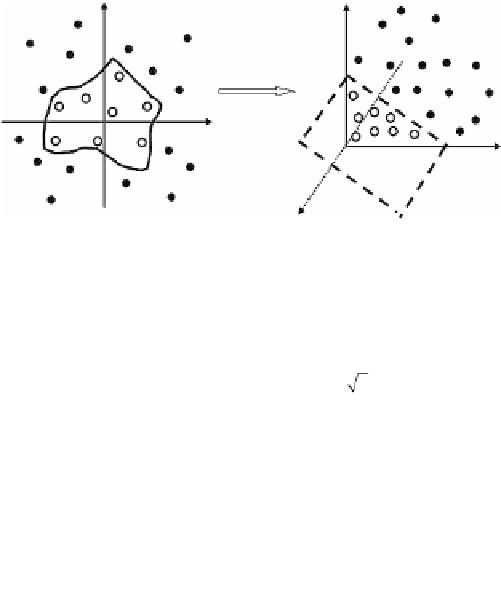
FIGURE 18.1 Diagram of nonlinear mapping in SVC. In order to classify the two classes

of points—black and white dots—in the original space, the red nonlinear classifier is
needed, as shown on the left. However, if we use the nonlinear mapping to map the
original data space to a high-dimensional feature space , that is mapping
to through , (for example, ), the points would be
able to be separated with a linear hyperplane, as shown on the right.

ℜ

2

Φ

x

ℜ

2

ℜ

3

Φ()

xz

xz = Φ Φ() ( , , ) ( , = =

12 3

z z x xxx

2

2 , )

2 12

The SVR training process can be formulated as a problem of finding an optimal set
of Lagrange multipliers α ∀∈ i [, 1 M ] , by maximizing the SVR objective function

i

M M M M

1
2

∑ ∑ =1 ∑ ∑

O =− ε | α | + y α − αα K x (, x ) (18.2)

i ii i j i j

i = 1 i i = 1 j = 1

subject to

1. linear constraints,

M

∑

α i = 0 , (18.3)

i = 1

and

2. box constraint,

−≤ ≤ ∀∈ C α C , i [ , 1 M ] (18.4)

i

x i

Here, α is the Lagrange multiplier associated with each training example ,

i

and ε in Equation 18.2 is the insensitivity value, meaning that training error below

ε is ignored. Figure 18.2 depicts the situation graphically for an ε -insensitivity

loss function L given by:

ε

0 for | fx ( ) −< y | ε

L =

ε

|() fx − y | − ε otherwise