Fundamentals of Data Analysis Methods in Functional MRI - Advance Image Processing in Magnetic Resonance Imaging - page 475

Spatial smoothing

Spatial smoothing

13 13

− 8.00 − 8.00

3.20 3.20

− −

8.00 8.00

3.20
t (123)
p < 0.001749

3.20
t (123)
p < 0.001749

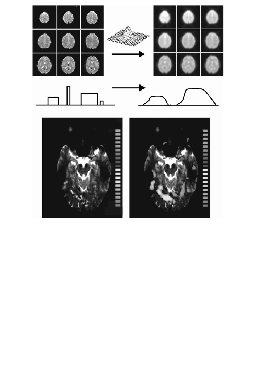
FIGURE 15.3 Spatial smoothing. Top row: Functional time series before (left) and after
(right) spatial filtering with a 3-D Gaussian smoothing kernel (FWHM = 3 voxels). Middle
row: Schematic representation of the effects of spatial smoothing on brain activation. For
simplicity, space is represented on a 1-D axis. Note that “activated” regions with a small
spatial extension may disappear after spatial smoothing. Lower row: Activation map
before (left) and after (right) spatial smoothing with a 3-D Gaussian smoothing kernel
(FWHM = 3 voxels).

MR signal drifts and physiological fluctuations at low temporal frequencies
are always present in fMRI time series and have to be corrected by linear

detrending or, more generally, by high-pass temporal filtering (see Figure 15.4 )

[18-21]. If the temporal sampling rate used for functional scanning (volume
repetition time) is sufficiently short, systematic physiological noise linked to the
cardiac and respiratory cycles can be eliminated using band-reject [20] or least-
mean-square (LMS) adaptive filters [21].