Image Processing Reference
In-Depth Information
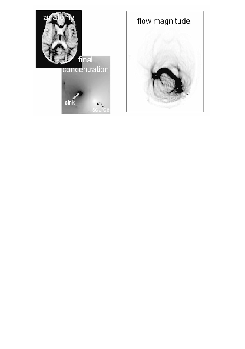
FIGURE 13.12
Results of solving Equation 13.26 for the steady-state heat distribution.
The temperature (labeled as concentration) and the steady-state flow magnitude demon-
strate the flow from the source to the sink. In the temperature image, the source is bright
and the sink is dark; in the flow image, dark means high flow magnitude. The grayscale
image on the left, a nondiffusion-weighted image, shows the corresponding anatomy.
has large magnitude. We calculate the weights in the mask as the linear shape
measure at each voxel, which lies in the range of zero to one [24,25]
λλ
λ
−
1
2
c
l
=
.
(13.28)
1
In addition, we remove negative eigenvalues to ensure that each tensor is a
positive definite matrix. We set a small positive lower bound for the eigenvalues
to guarantee that the tensors are invertible, which is necessary when utilizing
them as local metric descriptors as described later. Setting the negative eigenval-
ues to zero would give the closest positive semidefinite tensor in the least-squares
sense, but would not ensure invertibility.
Concentration or heat flow between regions:
In this experiment, we solve for
the steady-state concentration or heat distribution in the tensor field, with bound-
ary conditions of one source and one sink. The maximal flow is found as expected
along the strong anatomical path between the source and sink, the corpus callo-
sum. Figure 13.12 displays the steady-state concentration and flow.
13.7
METHOD TWO: DISTANCE-BASED
CONNECTIVITY
This method allows us to relate geodesic paths to connectivity, and investigate
paths from one point or region outward to the entire brain.


Search WWH ::

Custom Search