Basic Physics of MR Signal and Image Generation - Advance Image Processing in Magnetic Resonance Imaging - page 30

Considering the following substitution:

k =∆

=

γ
γ

n tG

x x

(1.44)

k t G

y G y

the formula in Equation 1.43 can be rewritten as:

∞ ∞

∫ ∫

− i (xk + yk )

s k ,k ( ) = c ρ ( x,y e ) dxdy (1.45)

x y

xy

−∞ −∞

This shows that the data matrix s(k x , k y ) is a sampling of the Fourier coefficients
of the function (x, y). Therefore, by applying a two-dimensional inverse Fourier

transform to the data s(n, m), the result will be an estimate of the function

ρ

(x, y).
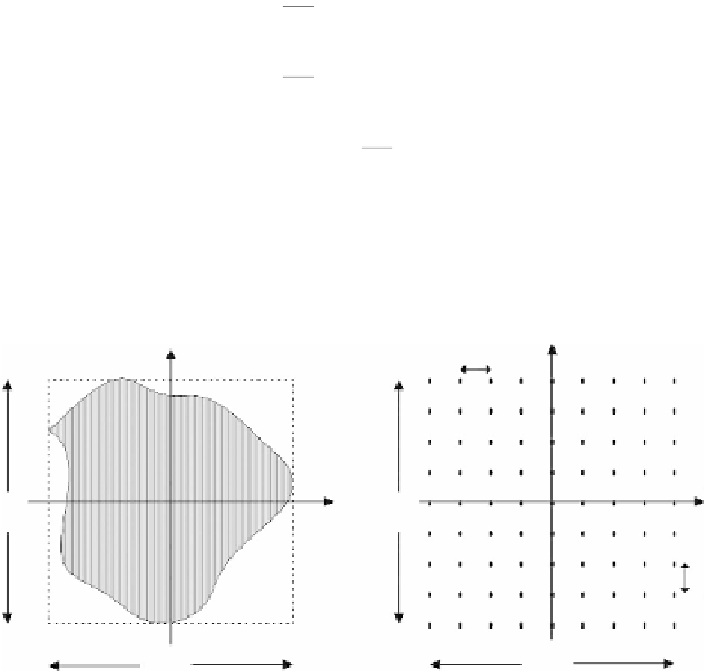
Several parameters of interest in the k-space can be defined in terms of
parameters described in the pulse sequence. The sample spacing and width of
the k-space are:

ρ

γ
π
γ
π

∆ k = Gt ∆

x x

2

∆ k = Gy ∆

y

2

y

(1.46)

γ
π

WNk = ∆ = GT

kx x x x

2

= γ
π

WM = ∆ k 2 G t

ky y y ,max G

2

k x k y

y

W y W ky

x

k x

k y

W kx

W x

FIGURE 1.15 Sampling parameters of k -space.