Principles of MR Spectroscopy and Chemical Shift Imaging - Advance Image Processing in Magnetic Resonance Imaging - page 379

TE/2 TE/2

90 180

rf

τ

G

N

ADC

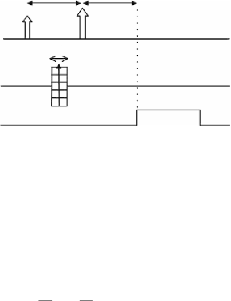
FIGURE 11.12 The scheme of the 1-D spin-echo CSI sequence.

After application of the refocusing pulse at time TE, data are sampled as a second
part of the spin echo.
The whole sequence is repeated N times with repetition time TR, while the
gradient strength G is changed in N equidistant steps

∆ G from the value G min = −

∆ G(N/21) as depicted in Figure 11.12.

Denoting G l as the gradient strength of the l-th phase-encoding step and
introducing variable k l

GN/2 to G max = ∆

γ
π τ

γ
π τ

k = G = l ∆ G l =− N N / .... 2 / 2 − 1 (11.3)

l l

2 2

the spatially dependent phase shift φ l (x) corresponding to l-th phase-encoding

step equals k l x.

Because the overall measured signal S(t) is the sum of all elementary signals
s(t,x) distributed along x axis, taking the additional phase into account, we can
for a measured signal write S(t, k l ) as a function of k l

φ l (x) = -2 π

∫

l x

St k (, ) = stxe (, )

− i 2π k

dx (11.4)

l

sample

The measured signal S(t, k l ) is the continuous Fourier transform (FT) of
the signals s(t, x) from elementary volumes. The positions of N voxels along
the x axis can be reconstructed by the inverse discrete Fourier transform
(DTF −1 ).

The 1-D sequence can be easily extended to 2-D ( Figure 11.13a ) or 3-D

(Figure 11.13b) variants. In 2-D and 3-D CSI, 2 and 3 orthogonal phase-encoding
gradients are applied, respectively. In reality, as shown in Figure 11.13, the
nonselective excitation pulse is often replaced by a frequency selective pulse